Embedding-Based Subsequence Matching in Large Sequence Databases
This doctoral dissertation by Panagiotis Papapetrou presents a novel approach to subsequence matching within large sequence databases, emphasizing embedding techniques to enhance efficiency. The work discusses various types of sequences, including time series and biological data, to demonstrate the applicability of the proposed methods. A key focus is on dynamic time warping (DTW) for measuring similarity, which allows for flexible alignment of sequences. The committee consists of esteemed scholars from reputable institutions, reviewing the innovative methodologies and results that advance the field of sequence analysis.

Embedding-Based Subsequence Matching in Large Sequence Databases
E N D
Presentation Transcript
Embedding-Based Subsequence Matching in Large Sequence Databases Doctoral Dissertation Defense Panagiotis Papapetrou Committee: • George Kollios • Stan Sclaroff • Margrit Betke • Vassilis Athitsos (University of Texas at Arlington) • Dimitrios Gunopulos (University of Athens) Committee Chair: Steve Homer
Subsequence matching • General Problem • Given: • Sequence S. • Query Q. • Similarity measure D. • Find the best subsequence of S that matches Q. • Types of Sequences: • Time Series. • Biological sequences (e.g. DNA).
Types of Sequences (1/2) • Time Series • Ordered set of events X = {x1, x2, …, xn}. • Weather measurements (temperature, humidity, etc). • Stock prices. • Gestures, motion, sign language. • Geological or astronomical observations. • Medicine: ECG, … X Q
Types of Sequences (2/2) • Strings • Defined over an alphabet Σ. • Text documents. • Biological sequences (DNA). • Near homology search: • Deviation from Q does not exceed a threshold δ (δ ≤ 15%). Q: TCTAGGGCA …ACTTAGCTGTAGTCGTTCTATGGCATATGCATGCTGATCTCGTGCGTCATG…
Searching Time Series Databases EBSM Embedding-Based Subsequence Matching • V. Athitsos, P. Papapetrou, M. Potamias, G. Kollios, and D. Gunopulos, “Approximate embedding-based subsequence matching of time series” SIGMOD2008
Time Series • A sequence of observations. • (X1, X2, X3, X4, …, Xm). • Each Xi is a real number, or a vector. • E.g., (2.0, 2.4, 4.8, 5.6, 6.3, 5.6, 4.4, 4.5, 5.8, 7.5) value axis time axis
Subsequence Matching in a Database • Naïve approach: brute-force search. query What subsequence of any database sequence is the best match for Q? database
Our Contribution • Partial reduction to vector search, via an embedding. • Quick way to identify a few candidate matches. query What subsequence of any database sequence is the best match for Q? database
How to Compare Time Series • Euclidean distance: • Matches rigidly along the time axis. • Dynamic Time Warping (DTW): • Allows stretching and shrinking along the time axis. • In our method, we use DTW.
(x2–y2)2 + (x1–y1)2 (x1–y1)2 DTW: Dynamic time warping (1/2) • Each cell c = (i, j) is a pair of indices whose corresponding values will be computed, (xi–yj)2, and included in the sum for the distance. • Euclidean path: • i = j always. • Ignores off-diagonal cells. Y yj xi X
(i-1, j) (i, j) (i-1, j-1) (i, j-1) (i, j) DTW: Dynamic time warping (2/2) b • DTW allows more paths. • Examine all valid paths: • Standard dynamic programming to fill in the table. • The top-right cell contains final result. shrink x / stretch y Y stretch x / shrink y X a
J-Position Subsequence Match X: long sequence What subsequence of X is the best match for Q … such that the match ends at position j? Q: short sequence
J-Position Subsequence Match position j X: long sequence What subsequence of X is the best match for Q … such that the match ends at position j? Q: short sequence
J-Position Subsequence Match position j X: long sequence What subsequence of X is the best match for Q … such that the match ends at position j? Q: short sequence
Sakurai, Y., Faloutsos, C., & Yoshikawa, M. “Stream Monitoring under the Time Warping Distance”, ICDE2007 Dynamic Programming (1/2) query (i, j) Q[1:i] Is matched * 0 0 0 0 0 0 0 0 0 0 0 0 0 0 0 database sequence X • For each (i, j): • Compute the j-position subsequence match of the first i items of Q.
Dynamic Programming (2/2) query (i, j) * 0 0 0 0 0 0 0 0 0 0 0 0 0 0 0 database sequence X • For each (i, j): • Compute the j-position subsequence match of the first i items of Q. • Top row: j-position subsequence match of Q. • Final answer: best among j-position matches. • Look at answers stored at the top row of the table.
query database sequence X Time Complexity • Assume that the database is one very long sequence. • Concatenate all sequences into one sequence. • O(length of query * length of database). • Does not scale to large database sizes.
Strategy: Identify Candidate Endpoints database sequence X
Strategy: Identify Candidate Endpoints database sequence X indexing structure
Strategy: Identify Candidate Endpoints database sequence X indexing structure query Q
Strategy: Identify Candidate Endpoints database sequence X candidate endpoints candidate endpoints indexing structure query Q
Strategy: Identify Candidate Endpoints database sequence X Candidate endpoint: last element of a possible subsequence match. candidate endpoints candidate endpoints indexing structure query Q
Strategy: Identify Candidate Endpoints database sequence X Use dynamic programming only to evaluate the candidates. candidate endpoints candidate endpoints indexing structure query Q
Vector Embedding database sequence X1 X2 X3 X4 X5 X6 X7 X8 X9 X10 X11 X12 X13 X14 X15
Vector Embedding database sequence X1 X2 X3 X4 X5 X6 X7 X8 X9 X10 X11 X12 X13 X14 X15 vector set
Vector Embedding database sequence X1 X2 X3 X4 X5 X6 X7 X8 X9 X10 X11 X12 X13 X14 X15 vector set query Q1 Q2 Q3 Q4 Q5
Vector Embedding database sequence X1 X2 X3 X4 X5 X6 X7 X8 X9 X10 X11 X12 X13 X14 X15 vector set query query vector Q1 Q2 Q3 Q4 Q5
Vector Embedding subsequence match database sequence • Embedding should be such that: • Query vector is similar to vector of match endpoint. X1 X2 X3 X4 X5 X6 X7 X8 X9 X10 X11 X12 X13 X14 X15 vector set query query vector Q1 Q2 Q3 Q4 Q5
Vector Embedding database sequence • Using vectors we identify candidate endpoints. • Much faster than brute-force search. X1 X2 X3 X4 X5 X6 X7 X8 X9 X10 X11 X12 X13 X14 X15 vector set query query vector Q1 Q2 Q3 Q4 Q5
Using Reference Sequences reference row |R| database sequence X • For each cell (|R|, j), DTW computes: • cost of best subsequence match of R ending in the j-th position of X. • Define FR(X, j) to be that cost. • FR is a 1D embedding. • Each (X, j) single real number.
Using Reference Sequences reference reference database sequence X query Q • Cell (|R|, |Q|), DTW computes: • cost of best subsequence match of R with a suffix of Q. • Define FR(Q) to be that cost.
Intuition About This Embedding • Suppose Q appears exactly as (Xi’, …, Xj). • If j-position match of R in X starts after i’, then: • Warping paths are the same. • FR(Q) = FR(X, j).
Intuition About This Embedding • Suppose Q appears inexactly as (Xi’, …, Xj). • If j-position match of R in X starts after i’: • We expect FR(Q) to be similar to FR(X, j). • Why? Little tweaks should affect FR(X, j) little.
Intuition About This Embedding • Suppose Q appears inexactly as (Xi’, …, Xj). • If j-position match of R in X starts after i’: • We expect FR(Q) to be similar to FR(X, j). • Why? Little tweaks should affect FR(X, j) little. • No proof, but intuitive, and lots of empirical evidence.
Intuition About This Embedding • If (Xi’, …, Xj) is the subsequence match of Q: • If j-position match of R in X starts after i’: • FR(Q) should (for most Q) be more similar to FR(X, j) than to most FR(X, t).
Multi-Dimensional Embedding • One reference sequence 1D embedding. R1 R1 database sequence X query Q
Multi-Dimensional Embedding • One reference sequence 1D embedding. • 2 reference sequences 2-dimensional embedding. R1 R1 database sequence X query Q R2 R2 database sequence X query Q
Multi-Dimensional Embedding • d reference sequences d-dim. embedding F. • If (Xi’, …, Xj) is the subsequence match of Q: • F(Q) should (for most Q) be more similar to F(X, j) than to most FR(X, t). R1 R1 database sequence X query Q R2 R2 database sequence X query Q
Filter-and-Refine Retrieval Offline step: • Compute F(X, j) for all j. Online steps, given a query Q: • Embedding step: • Compute F(Q). • Filter step: • Compare F(Q) to all F(X, j). • Select p best matches p candidate endpoints. • Refine step: • Use DTW to evaluate each candidate endpoint.
Filter-and-Refine Performance database sequence X • Accuracy: correct match must be among p candidates, for most queries. • Larger p higher accuracy, lower efficiency. candidate endpoints
Experiments - Datasets • 3 datasets from the UCR Time Series Data Mining Repository: • 50Words, Wafer, Yoga. • All database sequences concatenated one big sequence, of length 2,337,778. • Query lengths 152, 270, 426.
Experiments - Methods • Brute force: • Full DTW between each query and entire database sequence. • Similar to SPRING of Sakurai et al. • PDTW (Keogh et al. 2004, modified by us): • Makes time series smaller by factor of k. • Each chunk of k values replaced by their average. • Matching on smaller series used as filter step. • EBSM (our method). • 40-dimensional embedding.
Experiments – Performance Measures • Accuracy: • Percentage of queries giving correct results. • Efficiency: • DTW cell cost: cost of dynamic programming, as percentage of brute-force search cost. • Runtime cost: CPU time per query, as percentage of brute-force CPU time. • By definition, brute-force has: • accuracy 100%, • cell cost 100%, • runtime cost 100%.
Results – DTW Cell Cost highlights
Results – Running Time highlights
Conclusions on EBSM • EBSM: Indexing method for subsequence matching of time series. • Embeddings fast filter step using vector search. • State-of-the-art results in our experiments. • No guarantees as DTW is non-metric. • Embedding-based techniques for subsequence matching are promising.
Reference-Based Alignment of Strings RBSA Reference-Based Sequence Alignment P. Papapetrou,V. Athitsos, G. Kollios, and D. Gunopulos, “Reference-Based Alignment of Large Sequence Databases” VLDB2009 (To Appear)
String Matching • Given: • S: collection of sequences defined over an alphabet Σ. • Q: query sequence defined over Σ. • D: similarity measure. • Find the most similar subsequence in S.
Our focus: DNA • S: a set of DNA sequences. • Q: DNA sequence • with a small deviation from the database match. • within δ |Q|, for δ ≤ 15%. • can be large (up to 10,000 nucleotides).
The Edit Distance [Levenshtein et al.1966] • Measures how dissimilar two strings are. • ED (A,B) = minimum number of operations needed to transform A into B. • Operations = [insertion, deletion, substitution]. • Example: • A = ATC and B = ACTG A = A – T C ED (A,B) = 2 B = A C T G