Download
1 / 25
250 likes | 393 Vues
Segmentation of Vehicles in Traffic Video. Tun-Yu Chiang Wilson Lau. Introduction. Motivation In CA alone, >400 road monitoring cameras, plans to install more Reduce video bit-rate by object coding

E N D
Segmentation of Vehicles in Traffic Video Tun-Yu Chiang Wilson Lau
Introduction • Motivation • In CA alone, >400 road monitoring cameras, plans to install more • Reduce video bit-rate by object coding • Collect traffic flow data and/or surveillance e.g. count vehicles passing on highway, draw attention to abnormal driver behavior • Two different approaches to segmentation: • Motion Segmentation • Gaussian Mixture Model
Motion Segmentation • Segment regions with a coherent motion Coherent motion: similar parameters in motion model • Steps: • Estimate dense optic flow field • Iterate between motion parameter estimation and region segmentation • Segmentation by k-means clustering of motion parameters • Translational model use motion vectors directly as parameters
Optic Flow Estimation • Optic Flow (or spatio-temporal constraint) equation: Ix· vx + Iy· vy + It = 0 where Ix , Iy , It are the spatial and temporal derivatives • Problems • Under-constrained: add ‘smoothness constraint’ – assume flow field constant over 5x5 neighbourhood window weighted LS solution • ‘Small’ flow assumption often not valid: e.g. at 1 pixel/frame, object will take 10 secs (300 frames@30fps) to move across width of 300 pixels multi-scale approach
Multi-scale Optic Flow Estimation • Iteratively Gaussian filter and sub-sample by 2 to get ‘pyramid’ of lower resolution images • Project and interpolate LS solution from higher level which then serve as initial estimates for current level • Use estimates to ‘pre-warp’ one frame to satisfy small motion assumption • LS solution at each level refines previous estimates • Problem: Error propagation temporal smoothing essential at higher levels Level 2 1 pixel/frame Level 1 2 pixels/frame 4 pixels/frame Level 0 (original resolution)
Results: Optical flow field estimation • Smoothing of motion vectors across motion (object) boundaries due to • Smoothness constraint added (5x5 window) to solve optic flow equation • Further exacerbated by multi-scale approach • Occlusions, other assumption violations (e.g. constant intensity) ‘noisy’ motion estimates
[vx, vy, x, y, R, G, B] motion vectors pixel coordinates color intensities Segmentation • Extract regions of interest by thresholding magnitude of motion vectors • For each connected region, perform k-means clustering using feature vector: • Color intensities give information on object boundaries to counter the smoothing of motion vectors across edges in optic flow estimate • Remove small, isolated regions
Segmentation Results • Simple translational motion model adequate • Camera motion • Unable to segment car in background • 2-pixel border at level 2 of image pyramid (5x5 neighbourhood window) translates to a 8-pixel border region at full resolution
Segmentation Results • Unsatisfactory segmentation when optic flow estimate is noisy • Further work on • Adding temporal continuity constraint for objects • Improving optic flow estimation e.g. Total Least Squares • Assess reliability of each motion vector estimate and incorporate into segmentation
Per-pixel model Each pixel is modeled as sum of K weighted Gaussians. K = 3~5 The weights reflects the frequency the Gaussian is identified as part of background Model updated adaptively with learning rate and new observation Gaussian Background Mixture Model
Matching Criterion If no match found: pixel is foreground If match found: background is average of high ranking Gaussians. Foreground is average of low ranking Gaussians Update Formula Update weights: Update Gaussian: Match found: No Match found: Replace least possible Gaussian with new observation. background New observation Matching and model updating foreground Segmentation Algorithm
Segmentation Result 1 • Background: “disappearing” electrical pole, blurring in the trees • lane marks appear in both foreground/background
Segmentation Result 2 Cleaner background: beginning of original sequence is purely background, so background model was built faster.
Segmentation Result 3 Smaller global motion in original sequence: Cleaner foreground and background.
affects how fast the background model incorporates new observation K affects how sharp the detail regions appears Parameters matter
Artifacts: Global Motion • Constant small motion caused by hand-held camera • Blurring of background • Lane marks (vertical motion) and electrical pole (horizontal motion)
Global Motion Compensation • We used Phase Correlation Motion Estimation • Block-based method • Computationally inexpensive comparing to block matching
Segmentation After Compensation • Corrects artifacts before mentioned • Still have problems: residue disappears slower even with same learning rate
Constant repetitive motion (jittering) High contrast between neighborhood values (edge regions) The object would appear in both foreground and background Mixture model fails when …
Use block-based Phase Correlation Function (PCF) to estimate translation vectors. Phase Correlation Motion Estimation
Our Experiment • Obtain test data • We shoot our own test sequences at intersection of Page Mill Rd. and I-280. • Only translational motions included in the sequences • Segmentation • Tun-Yu experimented on Gaussian mixture model • Wilson experimented on motion segmentation