Download
1 / 49
510 likes | 736 Vues
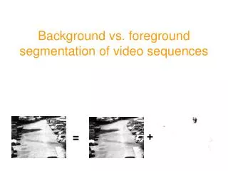
Background vs. foreground segmentation of video sequences. +. =. The Problem. Separate video into two layers: stationary background moving foreground Sequence is very noisy; reference image (background) is not given. Simple approach (1). background. temporal median. temporal mean.

E N D
Background vs. foreground segmentation of video sequences + =
The Problem • Separate video into two layers: • stationary background • moving foreground • Sequence is very noisy; reference image (background) is not given
Simple approach (1) background temporal median temporal mean
threshold Simple approach (2)
Variational approach Find the background and foregroundsimultaneously by minimizing energy functional Bonus: remove noise
[0,tmax] Notations given need to find C(x,t) background mask(1 on background, 0 on foreground) N(x,t) original noisy sequence B(x) background image
Energy functional: data term B N B - N C
Energy functional: data term • Degeneracy:can be trivially minimized by • C 0 (everything is foreground) • B N (take original image as background)
Energy functional: data term original images should be close to the restored background imagein the background areas there should be enough of background
Energy functional: smoothness For background image B For background mask C
Edge-preserving smoothnessRegularization term Quadratic regularization [Tikhonov, Arsenin 1977] ELE: Known to produce very strong isotropic smoothing
Edge-preserving smoothnessRegularization term Change regularization ELE:
n Edge-preserving smoothnessRegularization term Change the coordinate system: ELE: across the edge along the edge Compare:
Edge-preserving smoothnessRegularization term Conditions on Weak edge (s +0) (s) Isotropic smoothing (s) is quadratic at zero s
Edge-preserving smoothnessRegularization term Conditions on Strong edge (s +) • no smoothing across the edge: • more smoothing along the edge: (s) Anisotropic smoothing (s) does not grow too fast at infinity s
Edge-preserving smoothnessRegularization term Conclusion Using regularization term of the form: we can achieve both isotropic smoothness in uniform regions and anisotropic smoothness on edges with one function
Edge-preserving smoothnessRegularization term Example of an edge-preserving function:
Edge-preserving smoothnessSpace of Bounded Variations Even if we have an edge-preserving functional: if the space of solutions{u}contains only smooth functions, we may not achieve the desired minimum:
Edge-preserving smoothnessSpace of Bounded Variations which one is “better”?
Bounded Variation – ND case bounded open subset, function Variation of over φ where
Edge-preserving smoothnessSpace of Bounded Variations integrable (absolute value) and with bounded variation Functions are not required to have an integrable derivative … What is the meaning of u in the regularization term? Intuitively: norm of gradient |u|is replaced with variation |Du|
Total variation Theorem (informally): if uBV() then
Hausdorff measure area = 0 area > 0 How can we measure zero-measure sets?
Hausdorff measure 1) cover with balls of diameter 2) sum up diameters for optimal cover (do not waste balls) 3) refine: 0
Hausdorff measure Formally: For ARNk-dimensional Hausdorff measure of A up to normalization factor; covers are countable • HN is just the Lebesgue measure • curve in image: its length = H1 in R2
Total variation Theorem (more formally): if uBV() then u(x) u+ u- x0 x u+,u- - approximate upper and lower limits Su = {x; u+>u-} the jump set
Energy functional data term regularization for background image regularization for background masks
Total variation: example = perimeter = 4 Divide each side into n parts
Edge-preserving smoothnessSpace of Bounded Variations Small total variation(= sum of perimeters) Large total variation (= sum of perimeters)
Edge-preserving smoothnessSpace of Bounded Variations Small total variation Large total variation
Edge-preserving smoothnessSpace of Bounded Variations BV informally: functions with discontinuities on curves Edges are preserved, texture is not preserved: energy minimization in BV temporal median original sequence
Energy functional Time-discretized problem: Find minimum of E subject to:
Existence of solution Under usual assumptions 1,2: R+R+ strictly convex, nondecreasing, with linear growth at infinity minimum of E exists in BV(B,C1,…,CT)
(non-)Uniqueness is not convex w.r.t. (B,C1,…,CT)! Solution may not be unique.
Uniqueness But if c 3range2(Nt , t=1,…,T, x), then the functional is strictly convex, and solution is unique. Interpretation: if we are allowed to say that everything is foreground, background image is not well-defined
Finding solution BV is a difficult space: you cannot write Euler-Lagrange equations, cannot work numerically with function in BV. • Strategy: • construct approximating functionals admitting solution in a more regular space • solve minimization problem for these functionals • find solution as limit of the approximate solutions
Approximating functionals Recall: 1,2(s) = s2 gives smooth solutions Idea: replace i with i, which are quadratic at s 0 and s
Approximating problems has unique solution in the space • – convergence of functionals: ifE-converge to Ethen approximate solutions ofmin E converge to min E