Probability
Probability. Formal study of uncertainty The engine that drives statistics. Introduction. Nothing in life is certain We gauge the chances of successful outcomes in business, medicine, weather, and other everyday situations such as the lottery (recall the birthday problem). History.

Probability
E N D
Presentation Transcript
Probability Formal study of uncertainty The engine that drives statistics
Introduction • Nothing in life is certain • We gauge the chances of successful outcomes in business, medicine, weather, and other everyday situations such as the lottery (recall the birthday problem)
History • For most of human history, probability, the formal study of the laws of chance, has been used for only one thing: gambling
History (cont.) • Nobody knows exactly when gambling began; goes back at least as far as ancient Egypt where 4-sided “astragali” (made from animal heelbones) were used
Rule 1: Let Caesar win IV out of V times History (cont.) • The Roman emperor Claudius (10BC-54AD) wrote the first known treatise on gambling. • The book “How to Win at Gambling” was lost.
Approaches to Probability • Relative frequency event probability = x/n, where x=# of occurrences of event of interest, n=total # of observations • Coin, die tossing; nuclear power plants? • Limitations repeated observations not practical
Approaches to Probability (cont.) • Subjective probability individual assigns prob. based on personal experience, anecdotal evidence, etc. • Classical approach every possible outcome has equal probability (more later)
Basic Definitions • Experiment: act or process that leads to a single outcome that cannot be predicted with certainty • Examples: 1. Toss a coin 2. Draw 1 card from a standard deck of cards 3. Arrival time of flight from Atlanta to RDU
Basic Definitions (cont.) • Sample space: all possible outcomes of an experiment. Denoted by S • Event: any subset of the sample space S; typically denoted A, B, C, etc. Simple event: event with only 1 outcome Null event: the empty set F Certain event: S
Examples 1. Toss a coin once S = {H, T}; A = {H}, B = {T} simple events 2. Toss a die once; count dots on upper face S = {1, 2, 3, 4, 5, 6} A=even # of dots on upper face={2, 4, 6} B=3 or fewer dots on upper face={1, 2, 3}
Laws of Probability (cont.) 3. P(A’ ) = 1 - P(A) For an event A, A’ is the complement of A; A’ is everything in S that is not in A. S A' A
Birthday Problem • What is the smallest number of people you need in a group so that the probability of 2 or morepeople having the same birthday is greater than 1/2? • Answer: 23 No. of people 23 30 40 60 Probability .507 .706 .891 .994
Example: Birthday Problem • A={at least 2 people in the group have a common birthday} • A’ = {no one has common birthday}
Unions and Intersections S AÇB A B AÈB
Mutually Exclusive Events • Mutually exclusive events-no outcomes from S in common A Ç B = Æ S A B
Laws of Probability (cont.) Addition Rule for Disjoint Events: 4. If A and B are disjoint events, then P(A B) = P(A) + P(B)
5. For two independent events A and B P(A B) = P(A) × P(B)
Laws of Probability (cont.) General Addition Rule 6. For any two events A and B P(A B) = P(A) + P(B) – P(A B)
P(AÈB)=P(A) + P(B) - P(A Ç B) S AÇB A B
Example: toss a fair die once • S = {1, 2, 3, 4, 5, 6} • A = even # appears = {2, 4, 6} • B = 3 or fewer = {1, 2, 3} • P(A È B) = P(A) + P(B) - P(A Ç B) =P({2, 4, 6}) + P({1, 2, 3}) - P({2}) = 3/6 + 3/6 - 1/6 = 5/6
Laws of Probability: Summary • 1. 0 P(A) 1 for any event A • 2. P() = 0, P(S) = 1 • 3. P(A’) = 1 – P(A) • 4. If A and B are disjoint events, then P(A B) = P(A) + P(B) • 5. If A and B are independent events, then P(A B) = P(A) × P(B) • 6. For any two events A and B, P(A B) = P(A) + P(B) – P(A B)
Probability Models The Equally Likely Approach (also called the Classical Approach)
Assigning Probabilities • If an experiment has N outcomes, then each outcome has probability 1/N of occurring • If an event A1 has n1 outcomes, then P(A1) = n1/N
Product Rule for Ordered Pairs • A student wishes to commute to a junior college for 2 years and then commute to a state college for 2 years. Within commuting distance there are 4 junior colleges and 3 state colleges. How many junior college-state college pairs are available to her?
Product Rule for Ordered Pairs • junior colleges: 1, 2, 3, 4 • state colleges a, b, c • possible pairs: (1, a) (1, b) (1, c) (2, a) (2, b) (2, c) (3, a) (3, b) (3, c) (4, a) (4, b) (4, c)
Product Rule for Ordered Pairs • junior colleges: 1, 2, 3, 4 • state colleges a, b, c • possible pairs: (1, a) (1, b) (1, c) (2, a) (2, b) (2, c) (3, a) (3, b) (3, c) (4, a) (4, b) (4, c) 4 junior colleges 3 state colleges total number of possible pairs = 4 x 3 = 12
Product Rule for Ordered Pairs • junior colleges: 1, 2, 3, 4 • state colleges a, b, c • possible pairs: (1, a) (1, b) (1, c) (2, a) (2, b) (2, c) (3, a) (3, b) (3, c) (4, a) (4, b) (4, c) In general, if there are n1 ways to choose the first element of the pair, and n2 ways to choose the second element, then the number of possible pairs is n1n2. Here n1 = 4, n2 = 3.
Counting in “Either-Or” Situations • NCAA Basketball Tournament: how many ways can the “bracket” be filled out? • How many games? • 2 choices for each game • Number of ways to fill out the bracket: 263 = 9.2 × 10¹⁸ • Earth pop. about 6 billion; everyone fills out 1 million different brackets • Chances of getting all games correct is about 1 in 1,000
Counting Example • Pollsters minimize lead-in effect by rearranging the order of the questions on a survey • If Gallup has a 5-question survey, how many different versions of the survey are required if all possible arrangements of the questions are included?
Solution • There are 5 possible choices for the first question, 4 remaining questions for the second question, 3 choices for the third question, 2 choices for the fourth question, and 1 choice for the fifth question. • The number of possible arrangements is therefore 5 4 3 2 1 = 120
Efficient Methods for Counting Outcomes • Factorial Notation: n!=12 … n • Examples 1!=1; 2!=12=2; 3!= 123=6; 4!=24; 5!=120; • Special definition: 0!=1
Factorials with calculators and Excel • Calculator: non-graphing: x ! (second function) graphing: bottom p. 9 T I Calculator Commands (math button) • Excel: Paste: math, fact
Factorial Examples • 20! = 2.43 x 10¹⁸ • 1,000,000 seconds? • About 11.5 days • 1,000,000,000 seconds? • About 31 years • 31 years = 109 seconds • 1018 = 109 x 109 • 31 x 109 years = 109 x 109 = 1018 seconds • 20! is roughly the age of the universe in seconds
Permutations A B C D E • How many ways can we choose 2 letters from the above 5, without replacement, when the order in which we choose the letters is important? • 5 4 = 20
Permutations with calculator and Excel • Calculator non-graphing: nPr • Graphing p. 9 of T I Calculator Commands (math button) • Excel Paste: Statistical, Permut
Combinations A B C D E • How many ways can we choose 2 letters from the above 5, without replacement, when the order in which we choose the letters is not important? • 5 4 = 20 when order important • Divide by 2: (5 4)/2 = 10 ways
ST 101 Powerball Lottery From the numbers 1 through 20, choose 6 different numbers. Write them on a piece of paper.
North Carolina Powerball Lottery Prior to Jan. 1, 2009 After Jan. 1, 2009
Visualize Your Lottery Chances • How large is 195,249,054? • $1 bill and $100 bill both 6” in length • 10,560 bills = 1 mile • Let’s start with 195,249,053 $1 bills and one $100 bill … • … and take a long walk, putting down bills end-to-end as we go
Raleigh to Ft. Lauderdale… … still plenty of bills remaining, so continue from …
… Ft. Lauderdale to San Diego … still plenty of bills remaining, so continue from…
… San Diego to Seattle … still plenty of bills remaining, so continue from …
… Seattle to New York … still plenty of bills remaining, so continue from …
… New York back to Raleigh … still plenty of bills remaining, so …
Go around again! Lay a second path of bills Still have ~ 5,000 bills left!!

