Download
1 / 28
280 likes | 301 Vues
Explore the outer core, source of Earth's magnetic field, through the fluid convection of electrically conducting iron. Discover the complex field structure and dipole model in the mantle. Dive into the Glatzmaier-Roberts model to understand the magnetic field's dynamics and geomagnetic components. Learn how inclination and declination measurements determine the Virtual Geomagnetic Pole and North Pole locations. Uncover the significance of the Virtual Geomagnetic Pole in tracking Earth's magnetic field changes over time.

E N D
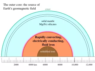
The outer core: the source of Earth’s geomagnetic field crust solid mantle Mg(Fe) silicates Rapidly convecting, electrically conducting, fluid iron solidified iron 2000 4000 km 6000 8000 10,000 12,000
crust solid mantle Mg(Fe) silicates • The geomagnetic dynamo: • turbulent fluid convection • electromagnetic interactions in fluid conductor • effects of rotation of earth solidified iron 2000 4000 km 6000 8000 10,000 12,000
A snapshot of the 3D magnetic field structure simulated with the Glatzmaier-Roberts geodynamo model. Magnetic field lines are blue where the field is directed inward and yellow where directed outward. The rotation axis of the model Earth is vertical and through the center. A transition occurs at the core-mantle boundary from the intense, complicated field structure in the fluid core, where the field is generated, to the smooth, potential field structure outside the core. The field lines are drawn out to two Earth radii. Magnetic field is wrapped around the "tangent cylinder" due to the shear of the zonal fluid flow.
90% of Earth’s geomagnetic field can be represented by a simple dipole located at the center of the earth! Field of a bar magnet revealed by iron filings
magnetic north pole The representation of the geomagnetic field as an earth-centered dipole magnetic field vector This is a planar section through the center of the earth, which intersects the surface as a “great circle” -p h magnetic equator +p two poles with pole strength -p and +p respectively, separted by a distance h form the dipole; its strength is measured by the product of p and h, termed the dipole moment. The magnetic poles are separated along a line, the dipole axis, which intersects the surface at the magnetic north and south poles. two poles with pole strength -p and +p respectively, separted by a distance h form the magnetic dipole; its strength is measured by the product of p and h, termed the dipole moment. The magnetic poles are separated along a line, the dipole axis, which intersects the surface at the magnetic north and south poles. axis of dipole magnetic south pole
magnetic north pole Field from dipole = vector composition of the fields from the two poles R -p h +p
magnetic north pole Field from dipole = vector composition of the fields from the two poles -p h R +p
magnetic north pole Field from dipole = vector composition of the fields from the two poles R -p h +p
magnetic north pole Field from dipole = vector composition of the fields from the two poles -p h R +p
magnetic north pole Field from dipole = vector composition of the fields from the two poles • Note the symmetry: • this section is the same for any great circle section that includes the dipole axis; • The magnetic field is always in such a section; • The horizontal component of the field is always along a great circle passing through the magnetic north pole. R -p h +p
geomagnetic north pole This great circle passes through the observation site and the magnetic north and south poles q = geomagnetic co-latitude q Inclination = I geomagnetic field vector measured at observation site -p magnetic equator +p Relationship between inclination, I and geomagnetic co-latitude, q: tan(I) = 2/tan(q) This is a key relationship in paleomagnetism: from measurement of I in a magnetized rock sample one can calculate the angular distance to the geomagnetic pole (the “virtual geomagnetic pole” or VGP). axis of dipole magnetic south pole
geomagnetic field components: F, I and D surface north east down
geomagnetic field components: F, I and D surface horizontal component north east I I = inclination, angle measured from surface in vertical plane to the geomagnetic field vector vertical component down
geomagnetic field components: F, I and D surface D north horizontal component east D = declination, angle measured in horizontal plane clockwise from North vertical component down
D as the angle between two great circles that intersect at the site location Great circle line of longitude between site location and north pole surface D north horizontal component east Horizontal component Points in the direction of magnetic North, along the great circle joining the site and the geomagnetic pole vertical component down
North Pole (NP) Measurement of D and I at a site location determines the location of the north geomagnetic pole if it is assumed that the field is entirely a simple earth centered dipole field. This determines the location of the “Virtual Geomagnetic Pole” or VGP site where magnetic field is measured
North Pole (NP) This is the longitudinal great circle that passes through the North Pole and the observation site VGP site where magnetic field is measured
North Pole (NP) VGP This is the great circle through the observation site and the VGP; it is the same great circle shown in sections in the preceding figures. site where magnetic field is measured
Why Virtual Geomagnetic Pole? 90% of the modern geomagnetic field is represented by a simple dipole at the center of the earth. The remaining 10%, the “non-dipole” components, have a more complicated spatial structure. Geomagneticians assume that in the past the earth’s field was also dominated by the dipole component. We can derive the location of the geomagnetic pole from an observation of inclination and declination at a site as indicated in the previous slides, by assuming that only the simple dipole is present, i.e., ignoring the non-dipole components. This produces an estimate of the location of the dipole component that we call the “virtual geomagnetic pole”. If we determine many VGP’s from many different locations and average the results, we obtain an estimate of the orientation of the dipole component of the field. This is the basic assumption for paleomagnetic determinations of past locations of areas relative to Earth’s rotation axis.
Locations of the north pole of the dipole component of the geomagnetic field from 1945-2000.
-30 to 800 BP 800 to 1940 BP 1940 to 3690 BP positions of the north magnetic pole during the past 3700 years. -30 to 3690 BP Average pole position for all data (94 poles): 88.4 N 23.8 W 1.6 degrees from geographic North Pole Calibrated radiocarbon years before present, (B.P, AD1950=0)
90 E VGP’s average Earth’s rotation axis! Polar projection showing VGP’s for igneous rocks at many sites, all dated at less than 20 million years old (too young to be significantly affected by plate motions). North Pole 180 0 30 N 15 N 90 W
Magnetization of rocks • Detrital Remanent Magnetization (DRM) • formed during deposition of sediments • locked in by compaction and lithification to sedimentary rock • relatively weak, but persistent over geological time scales
Magnetization of rocks • Thermo-remanent Magnetization (TRM) • formed in basic igneous rocks (e.g., basalt) upon cooling through Curie temperature • locked in for geological time scales upon further cooling • very strong and persistent
Magnetization of rocks Thermo-remanent Magnetization (TRM)
Magnetization of rocks • In both types of magnetization, the time of acquisiton of the stable magnitization must be • short • determinable (mainly via isotope geochemistry)
Lab questions 1. The southeastern coastal area of Alaska has a geology very different than areas farther inland, suggesting very different history – suggesting that the coastal area was terrane that had accreted onto Alaska in Late Cretaceous (100 Ma). Reliable paleomagnetic measurements taken on Early Jurassic (200 Ma) samples in the accreted terrane and in the interior are as follows: Accreted terrane: Declination = N10°W (= -10°), Inclination = +63° (magnetic field pointing downwards). Interior area: Declination = N10°E (= +10°), Inclination = +85° a. Calculate the latitudes of each area in the Early Jurassic. b. Calculate the average velocity of the accreted terrane relative to the interior area before it accreted (in units of centimeters/year) 2. Specify the location of the VGP's (location of virtual north magnetic pole) for the following cases: a. site latitude = 20.0 S; site longitude = 65.0 W; declination = 0.0; inclination = 0.0 b. site latitude = 20.0 S; site longitude = 30.0 E; declination = 0.0; inclination = 0.0 c. site latitude = 0.0 (equator); site longitude = 30.0 E; declination = 050 (N 50 E); inclination = 0.0 d. site latitude = 0.0 (equator); site longitude = 30.0 E; declination = 050 (N 50 E); inclination = -90 (magnetic vector pointing vertically upwards)