Download
1 / 34
340 likes | 494 Vues
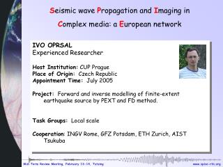
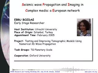
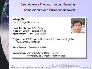
S eismic wave P ropagation and I maging in C omplex media: a E uropean network. Yilong Qin Early Stage Researcher Host Institution: IPG, Paris Place of Origin: Beijing, China Appointment Time: Jan. 2005 Project: A SPICE synthetic dataset to benchmark global tomographic methods

E N D
Seismic wave Propagation and Imaging in Complex media: a European network • Yilong Qin • Early Stage Researcher • Host Institution: IPG, Paris • Place of Origin: Beijing, China • Appointment Time: Jan. 2005 • Project:A SPICE synthetic dataset to benchmark global tomographic methods • Task Groups: Planetary Scales • Cooperation: Universitetet I Oslo, Norway • University of Utrecht, Netherlands
Content • Project Scope • Benchmark of benchmark • Final benchmark • Conclusions
Project Scope From The Reference Earth Model Website (http://mahi.ucsd.edu/Gabi/rem.html) There is general agreement about the location of long-wavelength structure. But the small-scale features still vary considerably from author to author
The benchmark of benchmark • Model build • Acquisition geometry • Computation • Synthetic data • Inversion results
Model build 3D model (Vs). Depth-independent Large-, medium- and samll-scale anomaly. Model parameters: isotropic Vp, Vs and density, gravity, attenuation 1D model (red) and PREM model (black) 1D reference model and 3D model
Acquisition geometry 27 events 256 receivers Distribution of events and station
Computation • 3D Coupling Spectral Elements and Modal Solution (CSEM) (Capdeville et al., ) • Z, N-S and E-W velocity component • Not consider the effect of ellipticity, crust, topography, ocean and rotation of real Earth. • 10500s records
Upper: comparison between CSEM and Normal-mode Lower: Source wavelet (left) and its spectrum (right)(minimum period 50s)
Synthetic data COYC FFC XMAS Comparison seismograms between 1D and 3D model
InversionAutomated multimode inversion based on time-frequency partition of waveform (Lebedev et al., 2005) Courtesy of S. Lebedev
The final benchmark • Acquisition geometry • Model build • Computation • Synthetic data
Distribution of stations and events. Near the location of red beach ball, three events are calculated.
Model build • Model parameters: P-wave isotropic average velocity, S-wave isotropic average velocity, Density, quality factor(Qmu), anisotropic parameter for vertically transverse anisotropic (xi, phi and eta) and the orientation of the crystal • 1D model • 3D variation • Crustal model • Topography and bathmetry
1D Valerie model • Anisotropic model (D” layer, upper mantle and transition zone) • Six layer (D’’, lower lower mantle, upper lower mantle, transition zone, upper mantle and crust) • boundary is 3480.0km, 3780.0km, 4700.0km, 5701.0km, 5971.0km, 6345.0km, 6371.0km.
P, S and density variation(release after blind test) • Random part: defined as spherical harmonic component. we have added mixture of adjacent layers over a depth interval of 250km. • The deterministic part: medium- and small-scale variation • S-wave and density variation are coupled with P-wave variation • Crystal with variable orientation of symmetry
Crustal model (smoothed CRUST2.0) Constant depth=26km Crustal model for Vs Crustal model for density The crust has a significant impact on the observed seismic data but, at the same time, is too thin to be resolved by them.
Topography and bathmetry (ETOPO5) The ocean are incorporated in the CSEM by introducing an equivalent load a the ocean floor(Dimitri Komatitsch and Jeroen Tromp, 2002)
Computation • Algorithm • coupling spectral element method (including the effect of anisotropy, gravity, attenuation, rotation, ocean, ellipticity, topography) • Computation time • Total hours is about 70000 CPU hours • Time step 0.35s, a compromise between numerical dispersion and computation cost. • Implementation • IPGP (Institut de physique du globe de Paris) • IDRIS (Institut du Développement et des Ressources en Informatique Scientifique) • CINES (Centre Informatique National de l'Enseignement Supérieur)
Mesh topography Coupling Spectral-element method (CSEM) Courtesy of Capdeville Ocean
Source wavelet spectrum wavelet An heavis wavelet with frequency up to 0.031Hz (minimum period 32s )
Numerical dispersion for maximum period 32s Comparison between normal-mode (black) and CSEM (red for 0.2s of time step , green for 0.4s time step) for minimum period of 32s.
Synthetic data • Three component (Z, N-S, E-W) velocity wavefield • Record length 10500s • Sampling rate is 1s • Format AH • No instrutment response • Add real noise from GEOSCOPE TAM
T L synthetic Z spectrum Station PAYG for event 09 (coupling between T, L and Z) for Valerie 1D model
Filtered ( >200s) Z component for station PAYG of event 09 Blue (3D model) and red (1D model)
Filtered (>200s) L component for station PAYG of event 09 Blue (3D model) and red (1D model)
Filtered >200s T component for station PAYG of event 09 Blue (3D model) and red (1D model)
Seismic noise for GEOSCOPE station TAM E and N component of noise is much stronger than Z component
download • http://www.ipgp.jussieu.fr/~qyl/benchmark_no_noise (about 1G) • http://www.ipgp.jussieu.fr/~qyl/benchmark_with_noise (about 1G) • README, 1D reference model, Source wavelet and dataset
Conclusions • Perform benchmark of benchmark • A complex 3D global anisotropic elastic model has been created • A high quality anisotropic elastic dataset has been created • Data and model (after blind test) are freely available
uses • phase velocity inversion • Waveform inversion • CMT inversion Limitations • Minimum period 32s
acknowledgement • SPICE • Service de Calcul Parallèle, in Institut de Physique du Globe de Paris • Sergei Lebedev (University of Utrecht)