Download
1 / 17
170 likes | 292 Vues
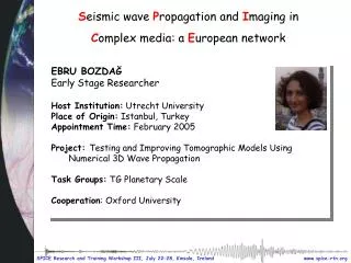
S eismic wave P ropagation and I maging in C omplex media: a E uropean network. EBRU BOZDA Ğ Early Stage Researcher Host Institution: Utrecht University Place of Origin: Istanbul, Turkey Appointment Time: February 2005

E N D
Seismic wave Propagation and Imaging in Complex media: a European network • EBRU BOZDAĞ • Early Stage Researcher • Host Institution: Utrecht University • Place of Origin: Istanbul, Turkey • Appointment Time: February 2005 • Project: Testing and Improving Tomographic Models Using Numerical 3D Wave Propagation • Task Groups: TG Planetary Scale • Cooperation: Oxford University
SPICE Crustal corrections predicted by ray theory and finite frequency theory compared to measured time shifts from SEM seismograms using Crust2.0 Ebru Bozdağ Jeannot Trampert Utrecht University, Utrecht, the Netherlands
Crustal corrections are important in surface wave tomography • Crustal structures have a strong effect on surface waves. • Inverting for crust and mantle is difficult. Therefore crustal corrections are preferred. • Phase delays from the crust are removed in surface wave tomography to identify mantle structure.
The objective Investigate how far • great circle approximation • exact ray theory and • finite frequency theory predict crustal corrections using theSEM (Komatitsch and Tromp, 2002) seismogramscomputed in1D(PREM)and 3D(PREM+Crust2.0)earth models.
VIC IJR XZNG CRT CMA IJR NCN SIR SOA SEP WIA Data generation Earthquakes & Stations 11 earthquakes 253 stations Synthetic seismograms using SEM • Synthetic seismograms from1D earth model PREM (Dziewonski and Anderson, 1981) • 3D crustal model Crust2.0 (Bassin et al., 2000) issuperimposed on top of PREM model and syntheticseismogramsare computed forPREM+Crust2.0 model
PREM Measure the phase of the cross-correlation PREM+Crust2.0 Measuring time shifts as a function of frequency Time-variable filter to extract the fundamental mode Rayleigh wave Phase correction to PREM seismograms Cross-correlation of the seismograms PREM+Crust2.0 - PREM PREM+Crust2.0 – PREM+Corr. Unwrap the phase
Methods used for crustal corrections Great Circle Approximation (GCA) Exact Ray Theory (ERT) Finite Frequency Theory (FFT)
Calculation of local phase velocity perturbations • At each grid point of Crust2.0, we superimpose the crustal model (plus topography) onto PREM and solve for the exact eigenfrequencies in that 1D earth model. • We thus generate exact local phase • velocities at each grid point which are used to calculate crustal corrections along rays.
A spherical harmonic expansion of the local phase velocities is used to simulate the smoothing of Crust2.0 in SEM Rayleigh, 40s Smoothing with spherical harmonic expansion Without smoothing dc/c0
Ray paths showing the time shifts computed for 150 s using GCA for one earthquake Time shifts from PREM+Crust2.0 – PREM seismograms time shift (s) Time shifts after correction (PREM+Crust2.0 -PREM+GCA)
Time shifts as a function of distance calculated for 150 s using GCA (l=40) 90% dt=±5.9 s 76% dt=±7.2 s 81% dt=±10.6 s 89% Black lines: average uncertainties of the measurements of Trampert & Woodhouse Blue bars: before correction (PREM+Crust2.0 - PREM) Red bars: after correction (PREM+Crust2.0 – PREM+GCA) dt=±19.4 s 92% dt=±22.7 s 96% dt=±27.8 s
Time shifts as a function of distance calculated for 40 s using GCA (l=40) 59% dt=±4.8 s 55% dt=±7.2 s 69% dt=±11.2 s 50% Black lines: average uncertainties of the measurements of Trampert & Woodhouse Blue bars: before correction (PREM+Crust2.0 - PREM) Red bars: after correction (PREM+Crust2.0 – PREM+GCA) dt=±17.8 s 62% dt=±20.8 s 78% dt=±24.8 s
Oceans-continents 150 s,GCA, l=40 Blue bars: before correction (PREM+Crust2.0 - PREM) Red bars: after correction (PREM+Crust2.0 - PREM+GCA)
Oceans-continents 40 s,GCA, l=40 Blue bars: before correction (PREM+Crust2.0 -PREM) Red bars: after correction (PREM+Crust2.0 - PREM+GCA)
Comparison of methods (150 s, l=40) GCA vs. FFT GCA vs. FFT (major arc) GCA vs. ERT FFT vs. ERT
Comparison of methods (40 s, l=40) GCA vs. FFT (major arc) GCA vs. FFT GCA vs. ERT FFT vs. ERT
Conclusions • No pronounced difference between GCA, ERT or FFT corrections • Corrections at 150 sec are better than at 40 sec • Corrections get worse as distance increases • We will now check if the imperfect corrections will lead to a detectable mantle signal