Download
1 / 39
390 likes | 548 Vues
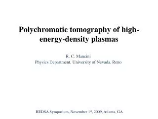
Polychromatic tomography of high-energy-density plasmas. R. C. Mancini Physics Department, University of Nevada, Reno. HEDSA Symposium, November 1 st , 2009, Atlanta, GA. Students and collaborators. Former students: Igor Golovkin (Prism), Leslie Welser (LANL)

E N D
Polychromatic tomography of high-energy-density plasmas R. C. Mancini Physics Department, University of Nevada, Reno HEDSA Symposium, November 1st, 2009, Atlanta, GA
Students and collaborators • Former students: Igor Golovkin (Prism), Leslie Welser (LANL) • Current students: Taisuke Nagayama, Heather Johns • Post-doc: Ricardo Florido • S. Louis, Computer Science Dep., UNR • R. Tommasini, N. Izumi, J. Koch, LLNL • J. Delettrez, F. Marshall, S. Regan, V. Smalyuk, LLE • J. Bailey, G. Rochau, SNL
Spatial structure of high-energy-density plasmas Implosion cores: significant progress has been made in three areas • Theory and modeling of x-ray line emission from tracers in plasmas: • collisional-radiative atomic kinetics, • detailed Stark-broadened line shapes including ion dynamic effects, • spectroscopic quality radiation transport. • Instrumentation and spectroscopic data: • GEKKO XII implosions: XMFC (toroidally bent crystal) x-ray imger1,2 • OMEGA indirect-drive implosions: MMI (pinhole array) x-ray imager3 • − Z implosions: TREX slit x-ray spectrometer • − OMEGA direct-drive implosions: DDMMI (pinhole array) x-ray imager • Data analysis methods need to solve an inversion problem: • quasi-analytic methods, • − multi-objective search & reconstruction driven by genetic algorithms, • − analysis of spatially-resolved line spectra. 1I. Golovkin, R. Mancini, S. Louis, Y. Ochi, K. Fujita, H. Nishimura, H. Shirga, N. Miyanaga, H. Azechi, R. Butzbach et al, Phys. Rev. Letters 88, 045002 (2002) 2Y. Ochi, I. Golovkin, R. Mancini, I. Uschmann, A. Sunahara, H. Nishimura, K. Fujita, S. Louis, M. Nakai, H. Shiraga, N. Miyanaga et al, Rev. Sci. Instrum. 74, 1683 (2003) 3L. Welser-Sherrill, R. Mancini, J. Koch, N. Izumi, R. Tommasini, S. Haan, D. Haynes, I Golovkin, J. MacFarlane, J. Delettrez et al, Phys. Rev. E 76, 056403 (2007)
Z-pinch dynamic-hohlraum experiments • Capsule implosion driven by a z-pinch dynamic-hohlraum1 • Nested W (Ti) wires, 240/120 wires, 40/20 mm diameter, 12 mm tall pinch • Radiation temperature 220 eV • Plastic capsule absorbs 20-40 kJ of X-ray energy • Plastic shell, diameter/wall thickness (mm/m): 2/50 z1155, 2/70 z1467 • Gas fill: 20-25 atm of D2 doped with 0.085 atm of Ar • At the implosion collapse, Ar line emission is observed for over 1 ns • Several quasi-orthogonal LOS: parallel to z-axis(trex1), and on planeperpendicular (trex2/trex5) to z-axis • Space- and time-resolved argon line spectra from implosion core • Argon K-shell line spectra from n = 2, 3, 4 and 5 in H- and He-like ions, and associated He- and Li-like satellites • Spectral resolution E/E 1000, spatial resolution X 30-50 m 1J. Bailey, G. Chandler, A. Slutz, I. Golovkin, P. Lake, J. MacFarlane, R. Mancini, T. Burris-Mog, G. Cooper, R. Leeper et al, Phys. Rev. Letters 92, 085002 (2004)
Z shot z1155: trex1f3 gated slit-imaged data X (m) trex1 Ly (Å) Ly He Ly He He • 2 mm/50 m, 20 atm D2 & 0.085 atm Ar. • Gated image data shows space-resolved • spectra recorded by the trex1 instrument. • A second instrument, trex2, recorded • similar data along an orthogonal LOS. • Each space-resolved lineout represents • a spatial integration over a core slice, • labeled by the coordinate X and with a • thickness given by the spatial resolution. X trex2 X
Z shot z1155: trex1f3, spatially-resolved spectra The line intensity distribution gradually changes as a function of the core slice coordinate X
Multi-objective spectroscopic analysis • Multi-objective data analysis driven by a Pareto Genetic Algorithm (PGA). • Search for Te and Ne spatial profiles that yield the best simultaneous and self-consistent fits to a set of spatially-resolved spectra recorded in Z-driven implosions. • The type of objective is the line intensity distribution, and the number of objectives is defined by the number of spectra in the dataset. • It relies on the Te and Ne dependence of the line intensity distribution over a broad photon energy range.
Core volume r X . LOS Core slice Image plane Problem set up and implementation • Geometry approximation: assume spherical geometry spatial structure is determined in terms of radial coordinate r. • Given Te(r) and Ne(r) in the source use a detailed atomic and radiation physics model to compute emissivity(r) and opacity(r).
Z shot z1155 trex1f3: set of self-consistent/simultaneous fits Simultaneous and self-consistent fits are systematically found for different LOS and time frame datasets
Z shot z1155: time-history of Te and Ne spatial profiles Analysis of four time frames recorded at the implosion collapse permits the reconstruction of time-history • Each frame is time-integrated over t = 0.5 ns each spatial profile • represents a time-average over 0.5 ns. • Earliest istrex1f2,latest istrex1f4; trex2f4 is in between trex1f3 and trex1f4. • Note:LOS of trex1 and trex2 are quasi-orthogonal. • During the period of observation, first, Te(r) and Ne(r) spatial profiles • increase in value. • Then, Te(r) values decrease while Ne(r) remains relatively high in value.
OMEGA direct-drive implosions • The amount of Ar has to be very small: • Not to change the hydrodynamics • To keep the optical depth of the Heb and Lyb (n=3-1 transitions) small • Laser: • 60 beams, several pulse shapes • Smoothing: 2D-SSD/DPP-SG4/DPR • Three identical DDMMI instruments: • DDMMI ≡ Direct-Drive Multi-Monochromatic x-ray Imager • Fielded along 3 quasi-orthogonal lines of sight (TIM3/TIM4/TIM5) • Record a collection of, gated, spectrally-resolved x-ray images of the implosion core
Spectrally-resolved core imaging with DDMMI DDMMI ≡ Direct-Drive Multi-Monochromatic x-ray Imager • A pinhole-array coupled to a multi-layer Bragg • mirror produces many quasi-monochromatic core • images, each one characteristic of a slightly • different photon energy range1,2 1B. Yaakobi, F.J. Marshall and D.K. Bradley, App. Optics 37, 8074 (1998) 2J.A. Koch, T.W. Barbee, Jr., N. Izumi, R. Tommasini, R.C. Mancini, L.A. Welser,,F.J. Marshall, Rev. Sci. Instrum. 76, 073708 (2005)
DDMMI data Lya Heb • Collection of gated, spectrally-resolved images • Time increases from F1 to F4 • Photon energy axis increases from left to right • Streaked data is used for time-correlation F1 F2 t F3 Lyb Heb F4 Lya hn (eV) 3200 5000
DDMMI data • Collection of gated, spectrally-resolved images • Photon energy axis increases from left to right • Resolution: • Spatial: ∆x = 10 mm • Spectral: E/∆E = 150 • From the array of spectrally-resolved images, one can extract: • Broad-band images • Narrow-band images • Space-integrated spectrum • Space-resolved spectra Lya Heb Lyb Narrow-band (Heb) Space-integrated Broad-band Space-resolved 3200 eV hn (eV) 5000 eV
140m Gated core images: broad-band and narrow-band based on argon spectral features Broad band OMEGA shot 49956, frame 3 (t3) Ly Broad band He Ly Ly He Broad band Ly He Ly Ly
140m Gated core images: broad-band and narrow-band based on argon spectral features Broad band OMEGA shot 49956, frame 4 (t4=t3+110ps) Ly Broad band He Ly Ly He Broad band Ly He Ly Ly
Set of space-resolved spectra from one-LOS OMEGA shot 49956 TIM4, Frame3
140m Volume determination based on three-LOS views OMEGA shot 49956, frame 3 x-y-z axes correspond to those defined in the chamber TIM4 • Consider a sphere of upper bound radius • Define boundaries (masks) based on broad-band images along each line of sight • Project these masks in space along each line of sight • Truncate the sphere with the intersections of projections • Get volume shape and size • Limitation: upper bound • The more LOS, the more accurate results TIM5 TIM3
Interpretation of SRS • Each space-resolved spectrum has temperature and • density information integrated along chord parallel • to LOS and perpendicular to the image plane
Interpretation of SRS • Each space-resolved spectrum has temperature and • density information integrated along chord parallel • to LOS and perpendicular to the image plane
Interpretation of SRS • Each space-resolved spectrum has temperature and • density information integrated along chord parallel • to LOS and perpendicular to the image plane • Each spatial region is located at the intersection of • three chords • Spatial regions are constrained by their contributions • to spatially-resolved spectra recorded along three LOS
Interpretation of SRS • Each space-resolved spectrum has temperature and • density information integrated along chord parallel • to LOS and perpendicular to the image plane • Each spatial region is located at the intersection of • three chords • Spatial regions are constrained by their contributions • to spatially-resolved spectra recorded along three LOS
Modeling: atomic kinetics and radiation transport • Physics model: Te and Ne spatial distribution SRS • ABAKO1: collisional-radiative atomic kinetics model • FAC for fundamental atomic data • Radiation transport effect on atomic kinetics using escape factors • Line shapes: detailed Stark, Doppler, and natural broadening effects • Continuum lowering based on Stewart-Pyatt approximation • Output: photon-, Te-, Ne-dependent emissivity (en) and opacity (kn) • Calculation of emergent intensity SRS • No symmetry assumptions, general 3D x-y-z space discretization grid • Numerically integrate radiation equation along chords en,kn 1R. Florido, R. Rodriguez, J. Gil, J. Rubiano, P. Martel, E, Minguez, R. Mancini, Phys. Rev E (2009, in press)
Synthetic-data test case Analysis method has to be tested: Do the sets of space-resolved spectra (SRS) recorded along three-LOS constrain the Te and Ne spatial distributions? Synthetic-data test case: • Step1: create random Te and Ne distributions in a 3D x-y-z grid Target Te and Ne distributions
Synthetic-data test case Analysis method has to be tested: Do the sets of space-resolved spectra (SRS) recorded along three-LOS constrain the Te and Ne spatial distributions? Synthetic-data test case: • Step1: create random Te and Ne distributions in a 3D x-y-z grid Target Te and Ne distributions • Step 2: synthetic data calculation target Te and Ne synthetic SRS
Synthetic-data test case Analysis method has to be tested: Do the sets of space-resolved spectra (SRS) recorded along three-LOS constrain the Te and Ne spatial distributions? Synthetic-data test case: • Step1: create random Te and Ne distributions in a 3D x-y-z grid Target Te and Ne distributions • Step 2: synthetic data calculation target Te and Ne synthetic SRS
Synthetic-data test case Analysis method has to be tested: Do the sets of space-resolved spectra (SRS) recorded along three-LOS constrain the Te and Ne spatial distributions? Synthetic-data test cases: • Step1: create random Te and Ne distributions in a 3D x-y-z grid Target Te and Ne distributions • Step 2: synthetic data calculation target Te and Ne synthetic SRS • Step 3: use search and reconstruction synthetic SRS find Te and Ne dist.
Synthetic-data test case Analysis method has to be tested: Do the sets of space-resolved spectra (SRS) recorded along three-LOS constrain the Te and Ne spatial distributions? Synthetic-data test Case: • Step1: create random Te and Ne distributions in a 3D x-y-z grid Target Te and Ne distributions • Step 2: synthetic data calculation target Te and Ne synthetic SRS • Step 3: use search and reconstruction synthetic SRS find Te and Ne dist. Uniqueness was checked
Synthetic-data test case Analysis method has to be tested: Do the sets of space-resolved spectra (SRS) recorded along three-LOS constrain the Te and Ne spatial distributions? Synthetic-data test case: • Step1: create random Te and Ne distributions in a 3D x-y-z grid Target Te and Ne distributions • Step 2: synthetic data calculation target Te and Ne synthetic SRS • Step 3: use search and reconstruction synthetic SRS find Te and Ne dist. Uniqueness was checked • Compare target Te and Ne dist. with extracted Te and Ne dist. Solution was checked Extracted Target
Results: OMEGA shot 49956 frame 3 • A total of 41 SRS were used to extract Te and Ne spatial structure • Te tends to be larger in central region Ne in the periphery • 3D asymmetries in the spatial structures are observed x = -21 mm x = 0 mm x = 21 mm Te (eV) Ne (cm-3)
Results: OMEGA shot 49956 frame 4 • A total of 23 SRS were used to extract Te and Ne spatial structure • Frame 4 is close to stagnation and the volume is smaller • Ne has increased while Te has decreased x = -21 mm x = 0 mm x = 21 mm Te (eV) Ne (cm-3)
Additional considerations • Analysis of streaked spectra recorded with SSCA yields space-averaged temperature and density for frame 3 and 4 that are consistent with the range of values in the spatial distributions extracted from the DDMMI data • Experimental Heb and Lyb narrow-band images reconstructed from DDMMI data compare well with the narrow-band images computed with the spatial distributions extracted from the analysis of SRS Heb Lyb Experiment Analysis Experiment Analysis Frame3 TIM5
Conclusions • Te and Ne spatial distributions have been extracted from the analysis of space-resolved spectra (SRS) obtained from spectrally-resolved images recorded with: (1) TREX and (2) three-identical DDMMI instruments fielded along quasi-orthogonal directions. • Analysis method: • two step search and reconstruction: PGA followed up by fine-tuning, • method was tested with synthetic data test case, • this method can be interpreted as polychromatic tomography: number of LOS is limited but there are multiple wavelengths associated with each LOS. • Related presentations: Monday 2PM, CP8 50 (T. Nagayama) and CP8 51 (R. Florido). • Work in progress: extraction of mixing spatial profiles. Work supported by DOE/NLUF Grant DE-FG52-09NA29042, LLNL and SNL
Z shot z1155 trex1f3: comparison of several methods Trends are consistent, and details can be interpreted in terms of methods’ approximations and assumptions • Note:X = core slice coordinate, r = radial coordinate. • Core slice analysis yields spatial averages over core slices of different sizes and • locations in the core (i.e. “non-local”). • Inversion method assumes spherical symmetry and optically thin and lines. • Multi-objective fits assumes only spherical symmetry.
DDMMI narrow-band image reconstruction 1 pixel column 1 pix Lyb 7 pix Lya Ti abs Lyg Heb Lyb Image • For a given narrow band range, pixels are collected and reassembled into the local positions of the image with their nearest centers as their reference points • Space-integrated spectrum can be computed by summing up intensities vertically 33 pix ∆E~70eV
TIM3 SSCA – MMI Time Correlation F1 F2 F3 F4 Shot # 49956 • X-ray streaked spectrometer • (SSCA) and gated imager (MMI) • record time-resolved data. • A time-correlation function • method is used to establish the • correspondence between • the time-axis of SSCA and the • F1, F2, F3 and F4 frames of MMI. • Good consistency is found using • the time-histories of Ly, He and • Ly spectral features. • The same method is used to time- • correlate SSCA with the LILAC 1D • hydro simulation. The label Rm • denotes the time of maximum • compression (i.e. minimum core • radius). Ly Lyβ Time correlation SSCA-MMI Heβ Lyα Rm
Search and reconstruction method • Pareto Genetic Algorithm (PGA)1 • Genetic Algorithms (GA) are fast and robust, search and optimization algorithms inspired by evolutionary biology • Pareto Genetic Algorithm (PGA) is the multi-objective version of GA • Search is initialized by random number generator (unbiased) • Uniqueness can be checked by changing random seed • Fine-tuning step: Levenberg-Marquardt non-linear least squares minimization method • Search and reconstruction method + physics model: SRS Te and Ne • Find Te and Ne spatial distributions that yield simultaneous and self-consistent fits to the given sets of SRS recorded along three-LOS • Two steps: Pareto genetic algorithm followed up by fine-tuning step The method is general and can be applied to other problems of multi-objective data analysis 1 I. Golovkin et al, Phys. Rev. Letters 88, 045002 (2002); L. Welser et al, J. Quant. Spec. Radiative. Transfer 99, 649 (2006); T. Nagayama et al. Rev. Sci. Instrum. 77, 10F525 (2006); T. Nagayama et al, Rev. Sci. Instrum. 79, 10E921 (2008)