Download
1 / 43
430 likes | 537 Vues
Study on variability of solar neutrino flux, including periodicities, available data sets, and analysis methods. Investigating the correlation with solar indices and potential oscillations.

E N D
VARIABILITY OF THE SOLAR NEUTRINO FLUX David Caldwell - UC Santa Barbara Jeff Scargle - NASA Ames Research Center Peter Sturrock, Guenther Walther - Stanford University Mike Wheatland - Sydney University S0306A06
SOLAR NEUTRINO PROBLEM STANDARD INTERPRETATION Standard Solar Model Neutrinos of Majorana type Effectively zero magnetic moment Flux Reduction due to Flavor Oscillation [MSW Effect ] Depends upon density Independent of magnetic field Since the solar density is spherically symmetric, the detected neutrino fluxes should be constant Time Variation is Incompatible with this Theory S0209A10
VARIABILITY TESTS Look for correlation between measured flux and some solar index such as sunspot number Examine variance of measurements, in comparison with simulations Examine histograms of measurements, in comparison with simulations Look for oscillations that can be identified with known solar oscillations Only #4 makes full use of the timing data S0209A11
SOLAR PERIODICITIES Hale cycle 22 years 0.046 cpy Sunspot cycle 11 years 0.09 cpy Howe oscillation 1.3 years 0.77 cpy Rieger oscillation 156 days 2.34 cpy Rieger-type oscillations 78 days 4.68 cpy 52 days 7.02 cpy Internal rotation - equatorial (sidereal) Radiative zone 13.9 +/-0.5 cpy Tachocline 13.7 to 14.6 cpy Convection zone 14.2 to 14.9 cpy Internal rotation - equatorial (synodic) Radiative zone 12.9 +/-0.5 cpy Tachocline 12.7 to 13.6 cpy Convection zone 13.2 to 13.9 cpy Plus harmonics of rotation rate S0209A09
SOLAR NEUTRINO FLUX VARIABILITYAVAILABLE DATA SETS • Homestake [Radiochemical - Chlorine] • GALLEX-GNO [Radiochemical - Gallium] • SAGE [Radiochemical - Gallium] • Super-Kamiokande [Cerenkov] S0205B12
SOLAR NEUTRINO FLUX VARIABILITYNOT YET AVAILABLE DATA SETS • Kamiokande, Kamiokande II [Cerenkov] • Sudbury Neutrino Observatory [SNO, Cerenkov] S0205B13
S0505B01 GALLEX AND GNO DATA ANALYSIS Histograms of flux values for (a) Gallex, and (b) GNO.
S0505B10 GALLEX AND GNO DATA ANALYSIS Histogram of flux values for Gallex and GNO combined
S0505B02 GALLEX AND GNO DATA ANALYSIS Histograms of (a) su for Gallex, (b) su for GNO, (c) sl for Gallex, (d) sl for GNO.
S0505B03 GALLEX AND GNO DATA ANALYSIS 5-point running means of the experimental flux estimates for Gallex and GNO
GALLEX AND GNO DATA ANALYSIS Likelihood functions for the flux for (a) Gallex and (b) GNO GALLEX GNO Flux estimates differ by 2 sigma P = 0.02 • S0505B04
GALLEX AND GNO DATA ANALYSIS TABLE 1 GALLEX DATA TABLE 2 GNO DATA Chi-Square = 4.90 P = 0.29 Chi-Square = 12.77 P = 0.012 Flux Probably Not Constant Flux Probably Constant • S0505B08
GALLEX AND GNO DATA ANALYSIS Normalized power spectrum, calculated using std(g) as the error term, for Gallex and GNO. • S0505B05
JOINT SPECTRUM STATISTIC From two (or more) power spectra, form a statistic analogous to a correlation statistic, defined so that it is distributed in the same way as a power spectrum. For gaussian random noise, We find that if S0205B04
GALLEX AND GNO DATA ANALYSIS Joint power spectrum formed from power at nu and at 2nu for Gallex and GNO. • S0505B07
R-MODES In a rotating fluid sphere, r-modes comprise oscillations for which the motion is mainly latitudinal. In the rotating frame, the oscillation frequencies are given by where is the rotation frequency, and l and m are the usual spherical harmonic indices. (The frequencies are independent of the index n.) These frequencies are close to the periods of Rieger-type oscillations. S0205B10
GALLEX AND GNO DATA ANALYSIS TABLE 3 • S0505B09
HOMESTAKE AND GALLEX-GNO • Lomb-Scargle spectrum of Homestake (left) and GALLEX-GNO (right) data in range 10 – 16 y-1 SXT01K07 S0205C06
SXT X-RAY DATA • Power spectra for SXT latitudes N60 and S60 (left) and Equator (right) SXT01K06 S0205C07
NEUTRINO AND X-RAY FLUX SPECTRA COMPARED Comparison of normalized probability distribution functions formed from power spectra: SXT N60&S60 (green), SXT Equator (red), Homestake (black), and GALLEX-GNO (blue) S0205B20 SXT01K05
SUPER-KAMIOKANDE Flux and Error Estimates in 10-day bins Neu02Y14 S0209A01
SUPER-KAMIOKANDE, 10-day bins Flux and Error Estimates (One Year Section) Neu02Y14 S0209A02
SUPER-KAMIOKANDE, 10-day bins Power Spectrum formed from Timing Schedule Very Strong Periodicity at 35.98 cpy Neu02Y06 S0209A05
SUPER-KAMIOKANDE, 10-day bins Power spectrum formed by likelihood analysis The biggest peak is at = 26.57 with S = 11.11 The second biggest peak is at = 9.41 with S = 7.33 The latter is an alias of the former, due to the peak at 35.98 in the power spectrum of the sampling schedule S0211A02
SUPER-KAMIOKANDE, 5-day bins LOMB-SCARGLE ANALYSIS S0505A08
SUPER-KAMIOKANDE, 5-day bins LIKELIHOOD ANALYSIS S0505A09
S0505A07 SUPER-KAMIOKANDE POWER SPECTRUM ANALYSIS Comparison of powers of top ten peaks for five analysis procedures: (1) basic Lomb-Scargle analysis, mean times; (2) basic Lomb-Scargle analysis, mean live times; (3) modified Lomb-Scargle analysis, mean live times, error data; (4) SWW likelihood method, start times, end times, and error data; (5) SWW likelihood method, start times, end times, mean live times, and error data. Only the peaks at 9.43 yr-1 and 43.72 yr-1 show a monotonic increase in power.
SUPER-KAMIOKANDE, 5-day bins S0505A10
SUPER-KAMIOKANDE, 5-day bins S0505A12
S0311A07 VARIABILITY OF THE SOLAR NEUTRINO FLUX It is therefore interesting to compare the power spectrum of the neutrino measurements with the power spectrum of the magnetic field at Sun center for the period of operation of Super-Kamiokande. We obtain the estimate 13.20 +/- 0.14 for the synodic rotation frequency (or 14.20 +/- 0.14 for the sidereal rotation frequency) of the magnetic field. This leads to the band 39.60 +/- 0.42 for the third harmonic of the synodic rotation frequency of the magnetic field. We see that peak C falls within this band. When we apply the shuffle test (Bahcall & Press 1991; Sturrock,Walther, &Wheatland 1997), randomly re-assigning flux and error measurements (kept together) to time bins, we find that only 5 cases out of 1,000 yield a power 8.91 or larger in the search band .
SUPER-KAMIOKANDE, 5-day bins S0505A13
S0311A01 VARIABILITY OF THE SOLAR NEUTRINO FLUX R-modes are retrograde waves that, in a uniform and rigidly rotating sphere, have frequencies as seen from Earth, where l and m are two of the usual spherical-harmonic indices, and nu is the sidereal rotation frequency.
S0311A02 VARIABILITY OF THE SOLAR NEUTRINO FLUX An observer co-rotating with the sphere would detect oscillations at the frequency (1) Since the mode frequency does not depend upon the radial index n, it seems likely that similar oscillations, with similar frequencies, could occur in thin spherical shells inside a radially stratified sphere.
S0311A03 VARIABILITY OF THE SOLAR NEUTRINO FLUX R-mode oscillations may modulate the solar neutrino flux by moving magnetic regions in and out of the path of neutrinos propagating from the core to the Earth. The resulting oscillations in the neutrino flux would be formed from combinations of the frequency with which an r-mode oscillation intercepts the core-Earth line and the frequency with which a magnetic structure intercepts the core-Earth line. These combinations will have the form (2) Where m’ , the azimuthal index for the magnetic structure, may be different from that of the r-mode.
S0311A04 VARIABILITY OF THE SOLAR NEUTRINO FLUX For m’ = m and for the minus sign, this yields the frequency of equation (1), and for the plus sign it yields (3) We may refer to this frequency for convenience as an “alias” of the frequency given by equation (1).
S0311A05 VARIABILITY OF THE SOLAR NEUTRINO FLUX For l = 2 and m = 2, and for the range of values of inferred from the magnetic-field data, we find that equation (1) leads us to expect an oscillation in the band 9.47 +/- 0.09, and equation (3) leads us to expect an oscillation in the band 43.33 +/- 0.47. We see that the peaks A and B fall within these two bands. On applying the shuffle test, we find only 6 cases out of 10,000 in which a peak with power 11.51 or larger occurs in the band 9.47 +/- 0.09, and only 5 cases out of 1,000 that yield a power 9.83 or larger in the band 43.33 +/- 0.47 .
SUPER-KAMIOKANDE, 5-day bins S0505A14
S0505C01 NEUTRINO PHYSICSINTERPRETATION OF SOLAR FLUX MODULATION Super-Kamiokande and SNO data show that Matter-Enhanced Neutrino Oscillations occur This must be the dominant process KamLAND data imply that similar oscillations occur involving rather than Solar and reactor data can be matched with Time-variation of the solar flux must therefore be a sub-dominant process.
S0505C02 NEUTRINO PHYSICSINTERPRETATION OF SOLAR FLUX MODULATION Time-variation points to the involvement of magnetic field. This indicates that modulation must be due to Resonant Spin Flavor Precession (RSFP) One possibility (Balantekin, Volpe) is but this effect is weak and occurs in the radiative zone. To get the correct shape of the time-averaged neutrino energy spectrum, we need
S0505C03 NEUTRINO PHYSICSINTERPRETATION OF SOLAR FLUX MODULATION The process cannot involve the three active neutrinos, since the width of the Z0 resonance limits the number of light, active neutrinos to three. Solar and reactor data require Atmospheric data require Hence a fourth neutrino is required. This must be sterile, to be consistent with Z0 data.
NEUTRINO PHYSICSINTERPRETATION OF SOLAR FLUX MODULATION Caldwell has proposed that solar-neutrino-flux time variation may be attributed to an RSFP process by which electron neutrinos are converted to sterile anti-neutrinos: via a transition magnetic moment. The sterile neutrino does not mix with other neutrinos, so this proposal is compatible with all limitations on sterile neutrinos. This model has been analyzed by Chauhan and Pulido. They find that • It gives an improved fit to time-averaged flux measurements • It eliminates an upturn that is expected, but not found, at lower energies in Super-Kamiokande and SNO data • It yields the correct magnitude of the modulation over the whole energy range • It yields the correct location of the effect (in the convection zone) S0505C04
SIGNIFICANCE FOR SOLAR PHYSICS OF THE VARIABILITY OF THE SOLAR NEUTRINO FLUX •Neutrinos may be used to probe the Sun’s internal magnetic field and internal dynamics • Variations are probably due to inhomogeneous magnetic structures with field strengths of order 105 Gauss in the outer radiative zone, the tachocline, or deep convection zone • The Rieger and related periodicities are due to internal r-mode oscillations, probably in or near the tachocline •Neutrino observations may give advance information of the development of the solar cycle S0205C10