Download
1 / 64
670 likes | 886 Vues
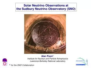
Solar Neutrino Observations at the Sudbury Neutrino Observatory (SNO). Alan Poon † Institute for Nuclear and Particle Astrophysics Lawrence Berkeley National Laboratory. † for the SNO Collaboration. Outline. Introduction — the Solar Neutrino Problem (SNP)

E N D
Solar Neutrino Observations at the Sudbury Neutrino Observatory (SNO) Alan Poon† Institute for Nuclear and Particle Astrophysics Lawrence Berkeley National Laboratory †for the SNO Collaboration
Outline Introduction — the Solar Neutrino Problem (SNP) Results from the Sudbury Neutrino Observatory Physics Implications Summary
Solar Neutrino Problem pp Chain:4p + 2e 4He +2ne+ 26.7MeV
Solar Neutrino Problem either Solar models are incomplete/incorrect or Neutrinos undergo flavor-changing oscillation In this talk, we will demonstrate that: Solar model prediction of the active 8B n flux is consistent with experiments AND Neutrinos change flavors while in transit to the Earth
Neutrino Oscillation 2 n Survival : Prob. Note: May also have resonant flavor conversion in matter — Mikheyev-Smirnov-Wolfenstein (MSW) effect
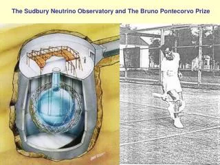
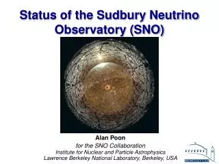
2 km to surface Sudbury Neutrino Observatory 1006 tonnes D2O 17.8m dia. PMT Support Structure 9456 20-cm dia. PMTs 56% coverage 12.01m dia. acrylic vessel 1700 tonnes of inner shielding H2O Urylon liner 5300 tonnes of outer shielding H2O NIM A449, 127 (2000)
p n + + + - CC d p e e n + + + n NC d p n x x ES - - + + n e n e x x Detecting in SNO • Measurement ofneenergy spectrum • Weak directionality: CC • Measure total 8Bnflux from the sun • s(ne)= s(nm)= s(nt) NC • Low Statistics • Sf=f(ne)+0.154 f(nm+nt) • Strong directionality: ES
Smoking Guns for Flavor Changing Oscillation Measure: Oscillation to active flavor if: THIS TALK
What else can NC tell us? nx+ d n + p + nx SNO NC • ne disappearance and nm/t appearance in one experiment: • Direct measurement of the total active 8B n flux • No ambiguity in combining results from experimentswith different systematics (e.g. energy resolution) • Lowest En threshold (2.2 MeV) for real time experiments [No energy spectral information] SNO CC
June 2001 NC analysis Radius (R/RAV)3 Solar Neutrino Analysis (NC+CC+ES) • NC and Day-Night Analysis in Pure D2O • Energy: Teff > 5 MeV • Fiducial vol.: R < 550 cm E Threshold Low E Background T>5 MeV T>5.5 MeV T>6 MeV Energy ~8 PMT hits / MeV
NC Data Analysis Data (Similar to high E threshold CC analysis) Instrumental Bkg Cut + Reconstruction inefficiency + Cherenkov “likelihood” Low Energy Background Analysis • Energy response • Reconstruction • (vertex) Energy Cut + Fiducial Volume Cut • Reconstruction • (vertex+directional) Signal Decomposition: CC, NC, ES • Neutron response
Data Reduction Nov 2, 1999 to May 28, 2001 306.4 live days Day=128.5 days, Night=177.9 days [c.f. High energy CC paper: 240.9 live days, 1169 candidate events]
A neutrino candidate event Event Reconstruction: Vertex, Direction, Energy, Light Isotropy PMT Information: Positions, Charges, Times
Data Reduction Cuts • Removeinstrumental background using: • PMT time & charge distribution • Event time correlation • Veto PMT tag • Reconstruction information • Light isotropy & arrival timing Light isotropy measure Light arrival timing nsignal loss: < 3 events (95% CL) Residual instrumental bkg. contamination:
NC Data Analysis Data (Similar to high E threshold CC analysis) Instrumental Bkg Cut + Reconstruction inefficiency + Cherenkov “likelihood” Low Energy Background Analysis • Energy response • Reconstruction • (vertex) Energy Cut + Fiducial Volume Cut • Reconstruction • (vertex+directional) Signal Decomposition: CC, NC, ES • Neutron response
Energy Response • Calibration: • PMT & Optics • Normalized to16N [Eg=6.13 MeV] • Check with • 8Li [13 MeV b] • 252Cf[d(n,g), Eg=6.25 MeV] • 3H(p,g) [19.8 MeV g] DE/E = ± 1.21% Ds/s = + 4.5% Linearity = ±0.23%@ Ee=19.1 MeV
Event Reconstruction Example: Angular Resolution (16N far from source) Given: Hit PMTs’ positions & timing Determine event’s: (x,y,z) & (q,f) Fiducial volume determination (Ntarget=?) Separation of n signals from background Tools: Triggered g and b sources
NC Data Analysis Data (Similar to high E threshold CC analysis) Instrumental Bkg Cut + Reconstruction inefficiency + Cherenkov “likelihood” Low Energy Background Analysis • Energy response • Reconstruction • (vertex) Energy Cut + Fiducial Volume Cut • Reconstruction • (vertex+directional) Signal Decomposition: CC, NC, ES • Neutron response
Neutron Detection Efficiency Response vs 252Cf source position • Calibrate using 252Cf fission source (~3.8 n per fission) • Capture Efficiency • Total:29.90 ± 1.10 % • With energy14.38 ± 0.53 % • threshold & • fiducial volume • selections • (T>5 MeV, R<550 cm)
NC Data Analysis Data (Similar to high E threshold CC analysis) Instrumental Bkg Cut + Reconstruction inefficiency + Cherenkov “likelihood” Low Energy Background Analysis • Energy response • Reconstruction • (vertex) Energy Cut + Fiducial Volume Cut • Reconstruction • (vertex+directional) Signal Decomposition: CC, NC, ES • Neutron response
Low Energy Background (Overview) Daughters in U or Th chain • b decays • bg decays “Photodisintegration” (pd) g+ d n + p Indistinguishable from NC ! Technique:Radiochemical assay Light isotropy “Cherenkov Tail” Cause: Tail of resolution, or Mis-reconstruction Technique: U/Th calib. source Monte Carlo Must know U and Th concentration in D2O
Measuring the U and Th Concentration in “Water” I.Ex-situ (Radiochemical Assays) • Count daughter product decays: 224Ra, 226Ra, 222Rn II.In-situ (Low energy physics data) • Statistical separation of 208Tl and 214Bi using light isotropy
LE Background Summary For Te 5 MeV, R<550cm [c.f.: 2928 n candidates] 12% of the number of observed NC neutrons assuming standard solar model n flux
NC Data Analysis Data (Similar to high E threshold CC analysis) Instrumental Bkg Cut + Reconstruction inefficiency + Cherenkov “likelihood” Low Energy Background Analysis • Energy response • Reconstruction • (vertex) Energy Cut + Fiducial Volume Cut • Reconstruction • (vertex+directional) Signal Decomposition: CC, NC, ES • Neutron response
OR + Df Extracting the n Signals Max. Likelihood Fit • PDFs: • kinetic energyT, event location R3, • and solar angle correlation cosq
Signal Extraction Results Assume standard 8B n spectrum Null hypothesis: no neutrino flavor mixing +61.9 -60.9 CC1967.7events NC576.5events ES263.6events +49.5 -48.9 +26.4 -25.6
Flux Uncertainties (Shape constrained) % fCC fNC fmt
NCSNO (2002) ESSNO (2001) ESSNO (2002) CCSNO (2001) CCSNO (2002) Solar n Flux Summary 8B from CCSNO+ESSK (2001) Constrained CC shape 5.3s Unconstrained CC shape Null hypothesis rejected at 5.3s F(ne+nm+nt) F(ne) F(ne)+0.15F(nm+nt) STRONG Evidence for ne nm and/or nt
Note: Disappearance and Reappearance Solar Model predictions are verified: [in 106 cm-2 s-1]
Day Flux vs Night Flux Day Night • Day: cos qzenith>0 (128.5 days) • Night: cos qzenith<0 (177.9 days) • 8B shape constrained extraction NC ES CC in units of x106 cm-2 s-1
Day-Night Uncertainties % The day-night analysis is currently statistics limited
Global Solar n Analysis • Inputs: • 37Cl, latest Gallex/GNO, new SAGE, SK 1258-day day & night spectra • SNO day spectrum (total: CC+NC+ES+background) • SNO night spectrum (total: CC+NC+ES+background) • 8B floats free in fit, hep n at 1 SSM m2>m1 m1>m2 Global SNO Day and Night spectra
Global n Analysis Fit Results • SNO CC/NC measurement directly constrains the survival probability at high energy • forces LOW solution to confront the Ga experimental results: [Experimental results: SK=2.32x106 cm-2 s-1, Ga=72.0±4.5 SNU, Cl=2.56±0.23 SNU]
Neutrino Mixing: What do we know now? Atmospheric n Uai = CHOOZ Solar n LMA Present situation: Solar nemix with
CKM vs MNSP Contrast between VCKM (quark) and UMNSP (lepton) [B Big s=small ]
Present Status & Future of SNO The Salt Phase Neutral Current Detectors 3He proportional counters n3He p t • 2 tonnes of NaCl added to D2O • Higher n-capture efficiency • Higher event light output • Light isotropy differs from e- • Running since June 2001 • To be deployed in early 2003 • Event-by-event separation of n
SNO Summary • Newest SNO results : • • nenm or nt appearance at 5.3 s • • Total 8B n flux measured for En>2.2 MeV • SSM prediction for total active 8B n flux verified • Day-Night results consistent with MSW hypothesis • Global fit including the newest SNO results : • • LMA highly favored (Dm2 ~ 5.0 x 10⁻⁵ eV2) • • No “dark side” and not maximal mixing (m1>m2, tan2(q)<1) • • Predictions for Borexino & KamLAND The NC and Day-Night papers (in July 1 issue of PRL), along with a HOWTO guide on using the SNO results are available at the official SNO website: http://sno.phy.queensu.ca
The SNO Collaboration G. Milton, B. Sur Atomic Energy of Canada Ltd., Chalk River Laboratories S. Gil, J. Heise, R.J. Komar, T. Kutter, C.W. Nally, H.S. Ng, Y.I. Tserkovnyak, C.E. Waltham University of British Columbia J. Boger, R.L Hahn, J.K. Rowley, M. Yeh Brookhaven National Laboratory R.C. Allen, G. Bühler,H.H.Chen* University of California, Irvine I. Blevis, F. Dalnoki-Veress, D.R. Grant, C.K. Hargrove, I. Levine, K. McFarlane, C. Mifflin, V.M. Novikov, M. O'Neill, M. Shatkay, D. Sinclair, N. Starinsky Carleton University T.C. Anderson, P. Jagam, J. Law, I.T. Lawson, R.W. Ollerhead, J.J. Simpson, N. Tagg, J.-X. Wang University of Guelph J. Bigu, J.H.M. Cowan, J. Farine, E.D. Hallman, R.U. Haq, J. Hewett, J.G. Hykawy, G. Jonkmans, S. Luoma, A. Roberge, E. Saettler, M.H. Schwendener, H. Seifert, R. Tafirout, C.J. Virtue Laurentian University Y.D. Chan, X. Chen, M.C.P. Isaac, K.T. Lesko, A.D. Marino, E.B. Norman, C.E. Okada, A.W.P. Poon, S.S.E Rosendahl, A. Schülke, A.R. Smith, R.G. Stokstad Lawrence Berkeley National Laboratory M.G. Boulay, T.J. Bowles, S.J. Brice, M.R. Dragowsky, M.M. Fowler, A.S. Hamer, A. Hime, G.G. Miller, R.G. Van de Water, J.B. Wilhelmy, J.M. Wouters Los Alamos National Laboratory J.D. Anglin, M. Bercovitch, W.F. Davidson, R.S. Storey* National Research Council of Canada J.C. Barton, S. Biller, R.A. Black, R.J. Boardman, M.G. Bowler, J. Cameron, B.T. Cleveland, X. Dai, G. Doucas, J.A. Dunmore, A.P. Ferarris, H. Fergani, K. Frame, N. Gagnon, H. Heron, N.A. Jelley, A.B. Knox, M. Lay, W. Locke, J. Lyon, S. Majerus, G. McGregor, M. Moorhead, M. Omori, C.J. Sims, N.W. Tanner, R.K. Taplin, M.Thorman, P.M. Thornewell, P.T. Trent, N. West, J.R. Wilson University of Oxford E.W. Beier, D.F. Cowen, M. Dunford, E.D. Frank, W. Frati, W.J. Heintzelman, P.T. Keener, J.R. Klein, C.C.M. Kyba, N. McCauley, D.S. McDonald, M.S. Neubauer, F.M. Newcomer, S.M. Oser, V.L Rusu, R. Van Berg, P. Wittich University of Pennsylvania R. Kouzes Princeton University E. Bonvin, M. Chen, E.T.H. Clifford, F.A. Duncan, E.D. Earle, H.C. Evans, G.T. Ewan, R.J. Ford, K. Graham, A.L. Hallin, W.B. Handler, P.J. Harvey, J.D. Hepburn, C. Jillings, H.W. Lee, J.R. Leslie, H.B. Mak, J. Maneira, A.B. McDonald, B.A. Moffat, T.J. Radcliffe, B.C. Robertson, P. Skensved Queen’s University D.L. Wark Rutherford Appleton Laboratory, University of Sussex R.L. Helmer, A.J. Noble TRIUMF Q.R. Ahmad, M.C. Browne, T.V. Bullard, G.A. Cox, P.J. Doe, C.A. Duba, S.R. Elliott, J.A. Formaggio, J.V. Germani, A.A. Hamian, R. Hazama, K.M. Heeger, K. Kazkaz, J. Manor, R. Meijer Drees, J.L. Orrell, R.G.H. Robertson, K.K. Schaffer, M.W.E. Smith, T.D. Steiger, L.C. Stonehill, J.F. Wilkerson University of Washington
How to solve the Solar Neutrino Problem? PRL 55, 1534 (1985)
Recap [Te > 6.75 MeV] Result 1: nenm,t SK ES (1s) Excludes: pure nensterile at 3.1 s 1.6 s 3.3 s Result 2: Solar model predictions are verified
Bifurcated Analysis Bifurcated analysis • Use a subset of the Pass 0 cuts and the HLC as two independent cuts • Number of residual instrumental background event = K = y1y2fB • K < 3 events (95% CL) Pass Cut 1: a+c = a1fn + y1fB Pass Cut 2: a+b = a2fn + y2fB Pass Cuts 1&2: a = a1a2fn + y1y2fB Total Data: S= fn + fB ai=neutrino acceptance for cut i yi=leakage of background for cut I fn=number of neutrino events fB=number of background events
Charge Pulsers • Pulsed Laser • 16N • 3H(p,g)4He • 8Li • 252Cf • U/Th Background Electronic 337nm to 620 nm 6.13 MeV g’s 19.8 MeV g’s <13.0 MeV b’s neutrons 214Bi & 208Tl b-g’s Understanding the Detector Response Monte Carlo • Cherenkov production (e-, g) • Photon propagation and detection • Neutron transport and capture • Event Reconstruction Calibration
Energy Calibration Uncertainties Absolute Energy Calibration Uncertainties Energy Response functions
Neutron Capture Efficiency 252Cf source data Measured: n capture on d (uniform source) 29.9 ± 1.1 %
pd background from D2O, AV, H2O radioactivity [c.f. SSM ~ 2 detected n d-1] The photodisintegration background is small compared to the SSM expectation
U and Th in/on the Acrylic Vessel • Original Target (2 ppt): 60 mg Th or U • Bulk acrylic assayed (NAA) • Dust concentration on inner and outer surfaces measured prior to filling • Hot spot (“Berkeley Blob”) found in Cherenkov data Z vs X projection [c.f. SSM ~ 2 detected n d-1]
Cherenkov Tail — D2O • Monte Carlo of detector response well calibrated in the D2O region • Determine Cherenkov tail background due to D2O radioactivity by Monte Carlo, using the U and Th concentration obtained above. • MC predictions cross checked with a Th calibration source T>5 MeV, R<550cm:
Cherenkov Tail • Determined from U/Th source calibration and Monte Carlo • Consistent with expectation based on measured U and Th concentration For Te 5 MeV, R<550cm [c.f.: 2928 n candidates]