Download
1 / 5
50 likes | 209 Vues
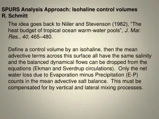
SPURS Analysis Approach: Isohaline control volumes R. Schmitt. The idea goes back to Niiler and Stevenson (1982), “The heat budget of tropical ocean warm-water pools”, J. Mar. Res. , 40 , 465–480.

E N D
SPURS Analysis Approach: Isohaline control volumes R. Schmitt The idea goes back to Niiler and Stevenson (1982), “The heat budget of tropical ocean warm-water pools”, J. Mar. Res., 40, 465–480. Define a control volume by an isohaline, then the mean advective terms across this surface all have the same salinity and the balanced dynamical flows can be dropped from the equations (Ekman and Sverdrup circulations). Only the net water loss due to Evaporation minus Precipitation (E-P) counts in the mean advective salt balance. This must be compensated for by vertical and lateral mixing processes.
3-D Shape of the 37.0 Isohaline Salinity Maximum Characteristics Blair – WHOI SSF
E-P Salt Fluxes Ekman+eddies Ekman+eddies Subduction+ vertical mixing By definition, =37.0, so mean advective input of salt reduces to (E-P) S. Mixing terms must flux this amount of salt back out of the volume. First results: Use of climatologies for E, P, T and S give reasonable vertical and horizontal diffusivities.
Isohaline volume budgets: issues What is the variability in the surface area of S >37.0 on seasonal and interannual times scales? (Aquarius, WOA…) What is variability of the volume? (Argo, …) What is the variability in E-P? What is time dependence of KV? (Seagliders, mooring…) What is the drifter salt flux across SSS=37.0? What is effect of seasonal cycle of mixed layer deepening on vertical fluxes? (moorings, Seagliders, ARGO floats…) What other Isohalines will work? (37.1, 37.2, 37.3…..) What do models show using this approach?
The Isohaline Control Volume: • The NA Salinity Maximum yields purely oceanic isohaline control volumes, providing a unique opportunity for budget calculations. • Can be used to integrate various data sets • The microstructure measurements (VMP, T-Gliders, Seagliders) can estimate the amount of vertical mixing, allowing for estimates of lateral diffusivities. • Increased vertical resolution should be possible using other isohaline surfaces. • Lateral mixing mechanisms may be quantified in the rich set of SPURS mooring, float, drifter and glider data. • The isohaline control volume is a promising integrating approach to pull together the diverse SPURS observations. • Many interesting questions arise: Seasonal and inter-annual variability of the volume, long term trends, specific mixing mechanisms…. • I need your help!