Download
1 / 77
2.44k likes | 4.96k Vues
Chapter 5 Time-Domain Analysis of Control Systems. Automatic Control Systems, 9 th Edition F. Golnaraghi & B. C. Kuo. 0, p. 253. Overview. Find and discuss transient and steady state time response of a simple control system.

E N D
Chapter 5Time-Domain Analysis of Control Systems Automatic Control Systems, 9th Edition F. Golnaraghi & B. C. Kuo
0, p. 253 Overview • Find and discuss transient and steady state time response of a simple control system. • Develop simple design criteria for manipulating the time response. • Look at the effects of addinga simple gain or poles and zerosto the system transfer function and relate them to the concept of control. • Look at simple proportional, derivative, and integral controller design concepts in time domain.
1, p. 253 Sections 5-1 and 5-2 5-1 Introduction • Time response: 5-2 Typical Test Signals for the Time Response of Control Systems • Step-Function Input: Steady-state response Transient response
2, p. 255 Ramp- and Parabolic-Function Inputs • Ramp-Function Input: • Parabolic-Function Input:
3, p. 256 5-3 The Unit-Step Response and Time-Domain Specification Steady-state error: r yssr: reference input
4, p. 258 5-4 Steady-State Error • Definition: errorsteady-state error • Unity feedback system (H(s) = 1)
4, p. 259 Velocity Control System • A step input is used to control the system output that contains a ramp in the steady state.System transfer function:Kt = 10 volts/rad/sec • Closed-loop transfer function: • Unit step response ( R(s)=1/s ): • Steady-state error:Kt = 10 volts/rad/sec reference signal is 0.1t, not 1 (unit step input).
4, p. 260 Systematic Study of Steady-State Error Three Types of Control Systems • System with unity feedback: H(s) = 1 e = r y • System with nonunity feedback,but H(0) = KH = constant e = r/KH y • System with nonunity feedbackand H(s) has zeros at s= 0 of order N.
4, p. 260 Steady-State Error of Unity Feedback • Steady-state error: • ess depends on the number of poles G(s) has at s = 0. • Forward-path transfer function:system type = j System type (the type of the control system)
4, p. 261 Unity Feedback with Step Func. Input Step-function input:
4, p. 262 Unity Feedback with Ramp Func. Input Ramp-function input:
4, p. 263 Unity Feedback with Para. Func. Input Parabolic-function input:
4, p. 264 Table 5-1
4, p. 265 Example 5-4-2
4, p. 265 Example 5-4-2 (cont.)
4, p. 266 Relationship between Steady-State Error and Closed-Loop Transfer Function State-State Error: H(0) = KH • Error signal: • M(s) does not have any poles at s = 0: Reference signal
4, p. 267 Steady-State Error: H(0)=KH • Step-function input: R(s) = R/sess = 0 or • Ramp-function input: R(s) = R/s2
4, p. 268 Steady-State Error: H(0)=KH(cont.) • Parabolic-function input: R(s) = R/s3
4, p. 268 Example 5-4-3
4, p. 269 Example 5-4-4
4, p. 269 Example 5-4-4 (cont.) • Unit-step input:y(t) 1, ess 0 • Unit-ramp input:y(t) t0.8, ess0.8 • Unit-parabolic input:y(t)0.5t2 0.8t11.2, ess0.8t+11.2
4, p. 270 Example 5-4-5 • Unit-step input: 0.5
4, p. 270 Example 5-4-5 (cont.) • Unit-ramp input:error: • Unit-parabolic input:error: 0.4 0.4t + 2.6
4, p. 270 Steady-State Error:H(s) Has Nth-Order Zero at s = 0 • Reference signal: R(s)/KHsN • Error signal: R(s) = R/s
4, p. 271 Example 5-4-6
4, p. 272 Steady-State Error Caused by Nonlinear System Elements
4, p. 273 Steady-State Error Caused by Nonlinear System Elements (cont.)
5, p. 274 5-5 Time-Response of a Prototype First-Order System time constant
6, p. 275 5-6 Time-Response of a Prototype Second-Order System G(s) Characteristic equation: R(s) = 1/s (unit-step input)
6, p. 276 Unit-Step Responses Figure 5-14 Unit-step response of the prototype 2nd-order system with various damping ratios.
6, p. 277 Damping Ratio and Damping Factor • Characteristic equation: • Unit-step response: • controls the rate of rise or decay of y(t). damping factor ( 1/ time constant ) • Damping ratio:
6, p. 278 Natural Undamped Frequency • Natural undamped frequency: n • Damped (or conditional) frequency:
6, p. 279 Figure 5-16
6, p. 280 Classification of System Dynamics
6, p. 281 Step-Response Comparison (Fig. 5-18) overdamped critically overdamped underdamped
6, p. 281 Step-Response Comparison (cont.) undamped negative overdamped negative overdamped
6, p. 281 Maximum Overshoot y() is maximum when 1. t = , n = 1 The first overshoot isthe maximum overshoot
6, p. 282 Maximum Overshoot (cont.)
6, p. 283 Maximum Overshoot (cont.) The first overshoot (n = 1) is the maximum overshoot
6, p. 283 Maximum Overshoot (cont.)
6, p. 283 Delay Time The time required for the step response to reach 50% of its final value Set y(t) = 0.5 and solve for t • Approximation:
6, p. 284 Rise Time The time for the step response to reach from 10 to 90% of its final value. • Approximation:
6, p. 285 Settling Time: 0 < < 0.69 The time required for the step response to decrease and staywithin a specified percentage(2% or 5%) of its final value.
6, p. 287 Settling Time: > 0.69
6, p. 287 Settling Time
7, p. 289 5-7 Speed and Position Control of a DC Motor • Open-loop response:
7, p. 290 Speed of Motor Shaft: Open-Loop • La is very small e = La/Ra (motor electric-time constant) is neglected.Keff = Km/(RaB+KmKb): motor gain constantm = RaJm/(RaB+KmKb): motor mechanical time constant
7, p. 291 Time Response: Open-Loop Superposition: • TL(s)=0 (no disturbance and B=0) and Va(s)=A/s: • TL(s)=D/s and Va(s)=A/s: (t) A/Kb (t) A/KbRaD/KmKb
7, p. 291 Closed-Loop Response
7, p. 292 Speed of Motor Shaft: Closed-Loop • La= 0 • in = A/sandTL = D/s:steady-state response: 1/c c: system mechanical-time constant