Time Domain Representations of Linear Time-Invariant Systems

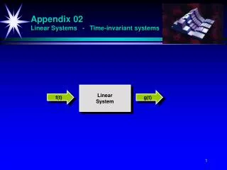
1. Time Domain Representations of Linear Time-Invariant Systems Chapter 2

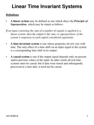
2. Introduction • Several methods can be used to describe the relationship between the input and output signals of LTI system. • Focus on system description that relate the output signal to the input signal when both are represented as function of time (time domain). • Impulse response defined as output of LTI system due to a unit impulse signal input applied at time t=0 or n=0.

3. Analysis of Continuous-Time Systems

4. H x(t) y(t) H (t) h(t) Impulse Response Let a system be described by and let the excitation be a unit impulse at time, t = 0. Then the response y is the impulse response h. d Since the impulse occurs at time t = 0 and nothing has excited the system before that time, the impulse response before time t = 0 is zero (because this is a causal system). After time t = 0 the impulse has occurred and gone away. Therefore there is no excitation and the impulse response is the homogeneous solution of the differential equation.

5. Impulse Response What happens at time, t = 0? The left side of the equation must be a unit impulse. The left side is zero before time t = 0 because the system has never been excited. The left side is zero after time t = 0 because it is the solution of the homogeneous equation whose right side is zero. These two facts are both consistent with an impulse. The impulse response might have in it an impulse or derivatives of an impulse since all of these occur only at time, t = 0. What the impulse response does have in it depends on the form of the differential equation.

6. Impulse Response Continuous-time LTI systems are described by differential equations of the general form, For all times, t < 0: If the excitation x(t) is an impulse, then for all time t < 0 it is zero. The response y(t) is zero before time t = 0 because there has never been an excitation before that time.

7. Impulse Response For all time t > 0: The excitation is zero. The response is the homogeneous solution of the differential equation. At time t = 0: The excitation is an impulse. In general it would be possible for the response to contain an impulse plus derivatives of an impulse because these all occur at time t = 0 and are zero before and after that time. Whether or not the response contains an impulse or derivatives of an impulse at time t = 0 depends on the form of the differential equation

8. Convolution • A systematic way to find systems respond. • Convolution integral for CT systems.

9. Exact Excitation Approximate Excitation The Convolution Integral

10. The Convolution Integral • All the pulses are rectangular and the same width, the only differences between pulses are when they occur and how tall they are. • So the pulse responses all have the same form except the delayed by some amount, to account for time of occurrence, and multiplied by a weighting constant, to account for the height.

11. The Convolution Integral Approximating the excitation as a pulse train can be expressed mathematically by or

12. The Convolution Integral Then, invoking linearity, the response to the overall excitation is (approximately) a sum of shifted and scaled unit pulse responses of the form

13. A Graphical Illustration of the Convolution Integral The convolution integral is defined by For illustration purposes let the excitation x(t) and the impulse response h(t) be the two functions below.

14. A Graphical Illustration of the Convolution Integral We can begin to visualize this quantity in the graphs below.

15. A Graphical Illustration of the Convolution Integral The functional transformation in going from h(t) to h(t - t) is

16. A Graphical Illustration of the Convolution Integral The convolution value is the area under the product of x(t) and h(t - t). This area depends on what t is. First, as an example, let t = 5. For this choice of t the area under the product is zero. Therefore if then y(5) = 0.

17. A Graphical Illustration of the Convolution Integral Now let t = 0. Therefore y(0) = 2, the area under the product.

18. A Graphical Illustration of the Convolution Integral The process of convolving to find y(t) is illustrated below.

19. Convolution Integral Properties Commutativity Associativity Distributivity

20. Cascade Connection System Interconnections If the output signal from a system is the input signal to a second system the systems are said to be cascade connected. It follows from the associative property of convolution that the impulse response of a cascade connection of LTI systems is the convolution of the individual impulse responses of those systems.

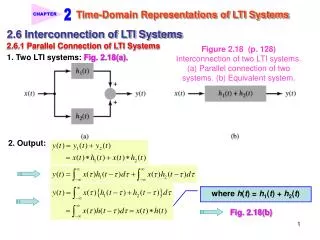
21. Parallel Connection System Interconnections If two systems are excited by the same signal and their responses are added they are said to be parallel connected. It follows from the distributive property of convolution that the impulse response of a parallel connection of LTI systems is the sum of the individual impulse responses.

22. Stability and Impulse Response A system is BIBO stable if its impulse response is absolutely integrable. That is if

23. Unit Impulse Response and Unit Step Response In any LTI system let an excitation x(t) produce the response y(t). Then the excitation will produce the response It follows then that the unit impulse response is the first derivative of the unit step response and, conversely that the unit step response is the integral of the unit impulse response.

24. Complex Exponential Response Let an LTI system be excited by a complex exponential of the form The response is the convolution of the excitation with the impulse response or

25. Analysis of Discrete-Time Systems

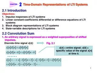
26. Impulse Response Discrete-time LTI systems are described mathematically by difference equations of the form For any excitation x[n] the response y[n] can be found by finding the response to x[n] as the only forcing function on the right-hand side and then adding scaled and time-shifted versions of that response to form y[n]. If x[n] is a unit impulse, the response to it as the only forcing function is simply the homogeneous solution of the difference equation with initial conditions applied. The impulse response is conventionally designated by the symbol h[n].

27. Impulse Response Since the impulse is applied to the system at time n = 0, that is the only excitation of the system and the system is causal. The impulse response is zero before time n = 0. After time n = 0, the impulse has come and gone and the excitation is again zero. Therefore for n > 0, the solution of the difference equation describing the system is the homogeneous solution.

28. System Response • Once the response to a unit impulse is known, the response of any LTI system to any arbitrary excitation can be found • Any arbitrary excitation is simply a sequence of amplitude-scaled and time-shifted impulses • Therefore the response is simply a sequence of amplitude-scaled and time-shifted impulse responses

29. Simple System Response Example

30. More Complicated System Response Example System Excitation System Impulse Response System Response

31. Convolution • A systematic way to find systems respond. • Convolution sum for DT systems. • Based on a simple idea, no matter how complicated an excitation signal is, it is simply a sequence of DT impulses. • Therefore, with the assumption that the impulse response to a unit impulse excitation occuring at time n=0 has already found, we will use the convolution technique to find system response.

32. The Convolution Sum The response y[n] to an arbitrary excitation x[n] is of the form where h[n] is the impulse response. This can be written in a more compact form called the convolution sum.

33. A Convolution Sum Example

34. A Convolution Sum Example

35. A Convolution Sum Example

36. A Convolution Sum Example

37. Convolution Sum Properties Convolution is defined mathematically by The following properties can be proven from the definition. Let then and the sum of the impulse strengths in y is the product of the sum of the impulse strengths in x and the sum of the impulse strengths in h.

38. Convolution Sum Properties (continued) Commutativity Associativity Distributivity

39. System Interconnections The cascade connection of two systems can be viewed as a single system whose impulse response is the convolution of the two individual system impulse responses. This is a direct consequence of the associativity property of convolution.

40. System Interconnections The parallel connection of two systems can be viewed as a single system whose impulse response is the sum of the two individual system impulse responses. This is a direct consequence of the distributivity property of convolution.

41. Stability and Impulse Response It can be shown that a BIBO-stable system has an impulse response that is absolutely summable. That is,

42. Unit Impulse Response and Unit Sequence Response In any LTI system let an excitation x[n] produce the response y[n]. Then the excitation x[n] - x[n - 1] will produce the response y[n] - y[n - 1] .

43. Complex Exponential Response Let an LTI system be excited by a complex exponential of the form The response is the convolution of the excitation with the impulse response or which can be written as