Download
1 / 35
360 likes | 556 Vues
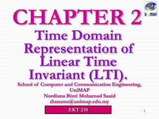
2. CHAPTER. Time-Domain Representations of LTI Systems. 2.11 Characteristics of Systems Described by Differential and Difference Equations. Complete solution: y = y ( n ) + y ( f ). y ( n ) = natural response,. y ( f ) = forced response. 2.11.1 The Natural Response.

E N D
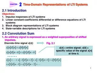
2 CHAPTER Time-Domain Representations of LTI Systems 2.11 Characteristics of Systems Described by Differential and Difference Equations Complete solution: y = y(n) + y(f) y(n) = natural response, y(f) = forced response 2.11.1 The Natural Response Example 2.24RCCircuit (continued): Natural Response The system In Example 2.17 is described by the differential equation Find the natural response of the this system, assuming that y(0) = 2 V, R = 1 and C = 1 F. <Sol.> 1. Homogeneous sol.: 2. I.C.: y(0) = 2 V y(n) (0) = 2 V c1 = 2 3. Natural Response:
2 CHAPTER Time-Domain Representations of LTI Systems Example 2.25First-OrderRecursive System (Continued): Natural Response The system in Example 2.21 is described by the difference equation Find the natural response of this system. <Sol.> 1. Homogeneous sol.: 2. I.C.: y[ 1] = 8 c1 = 2 3. Natural Response: The forced response is valid only for t 0 or n 0 2.11.2 The Forced Response The forced response is the system output due to the input signal assuming zero initial conditions.
2 CHAPTER Time-Domain Representations of LTI Systems The at-rest conditions for a discrete-time system, y[ N] = 0, …, y[ 1] = 0, must be translated forward to times n = 0, 1, …, N 1 before solving for the undetermined coefficients, such as when one is determining the complete solution. Example 2.26First-OrderRecursive System (Continued): Forced Response The system in Example 2.21 is described by the difference equation Find the forced response of this system if the input is x[n] = (1/2)nu[n]. <Sol.> 1. Complete solution: 2. I.C.: Translate the at-rest condition y[ 1] to time n = 0 y[0] = 1 + (1/4) 0 =1 3. Finding c1: c1 = 1
2 CHAPTER Time-Domain Representations of LTI Systems 4. Forced response: Example 2.27RCCircuit (continued): Forced Response The system In Example 2.17 is described by the differential equation Find the forced response of the this system, assuming that x(t) = cos(t)u(t) V, R = 1 and C = 1 F. From Example 2.22 <Sol.> 1. Complete solution: 2. I.C.: y(0) = y(0+) = 0 c = 1/2 3. Forced response:
2 CHAPTER Time-Domain Representations of LTI Systems 2.11.3 The Impulse Response Relation between step response and impulse response 2. Discrete-time case: 1. Continuous-time case: 2.11.4 Linearity and Time Invariance Forced response Linearity Natural response Linearity The complete response of an LTI system is not time invariant. Response due to initial condition will not shift with a time shift of the input. 2.11.5 Roots of the Characteristic Equation
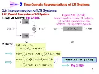
2 CHAPTER and The system is said to be on the verge of instability. Time-Domain Representations of LTI Systems Roots of characteristic equation Forced response, natural response, stability, and response time. ★ BIBO Stable: 1. Discrete-time case: 2. Continuous-time case: 2.12 Block Diagram Representations A block diagram is an interconnection of the elementary operations that act on the input signal. Three elementary operations for block diagram: • Scalar multiplication: y(t) = cx(t) or y[n] = cx[n], where c is a scalar. • Addition: y(t) = x(t) + w(t) or y[n] = x[n] + w[n]. • Integration for continuous-time LTI system: ; and a time shift for discrete-time LTI system: y[n] = x[n 1]. Fig. 2.32.
2 CHAPTER (a) (c) (b) Time-Domain Representations of LTI Systems Figure 2.32 (p. 162)Symbols for elementary operations in block diagram descriptions of systems. (a) Scalar multiplication. (b) Addition. (c) Integration for continuous-time systems and time shifting for discrete-time systems. Ex. A discrete-time LTI system: Fig. 2.33. Direct Form I: 1. In dashed box: (2.49) 2. y[n] in terms of w[n]:
2 CHAPTER Time-Domain Representations of LTI Systems (2.50) 3. System output y[n] in terms of input x[n]: Cascade Form (Direct Form I) (2.51) Figure 2.33 (p. 162)Block diagram representation of a discrete-time LTI system described by a second-order difference equation.
2 CHAPTER Time-Domain Representations of LTI Systems Direct Form II: 1. Interchange the order of Direct Form I. 2. Denote the output of the new first system as f[n]. Input: x[n] (2.52) 3. The signal is also the input to the second system. The output of the second system is (2.53) Fig. 2.35. Figure 2.35 (p. 164)Direct form II representation of an LTI system described by a second-order difference equation.
2 CHAPTER Time-Domain Representations of LTI Systems Block diagram representation for continuous-time LTI system: 1. Differential Eq.: (2.54) 2. Let v(0)(t) = v(t) be an arbitrary signal, and set v(n)(t) is the n-fold integral of v(t) with respect to time 3. Integrator with initial condition: Integrate N times to eq. (2.54) (2.55)
2 CHAPTER Time-Domain Representations of LTI Systems Ex. Second-order system: (2.56) (a) Figure 2.37 (p. 166)Block diagram representations of a continuous-time LTI system described by a second-order integral equation. (a) Direct form I. (b) Direct form II. (b)
2 CHAPTER Time-Domain Representations of LTI Systems 2.13 State-Variable Description of LTI Systems The state of a system may be defined as a minimal set of signals that represent the system’s entire memory of the past. Given initial point ni (or ti) and the input for time n ni (or t ti), we can determine the output for all times nni (or tti). 2.13.1 The State-Variable Description 1. Direct form II of a second-order LTI system: Fig. 2.39. 2. Choose state variables: q1[n] and q2[n]. 3. State equation: (2.57) (2.58) 4. Output equation: (2.59) 5. Matrix Form of state equation: (2.60)
2 CHAPTER Time-Domain Representations of LTI Systems Figure 2.39 (p. 167)Direct form II representation of a second-order discrete-time LTI system depicting state variables q1[n] and q2[n].
2 CHAPTER Time-Domain Representations of LTI Systems 6. Matrix form of output equation: (2.61) Define state vector as the column vector We can rewrite Eqs. (2.60) and (2.61) as (2.62) (2.63) where matrix A, vectors b and c, and scalar D are given by Example 2.28State-Variable Description of a Second-Order System Find the state-variable description corresponding to the system depicted in Fig. 2.40 by choosing the state variable to be the outputs of the unit delays. <Sol.>
2 CHAPTER Time-Domain Representations of LTI Systems Figure 2.40 (p. 169)Block diagram of LTI system for Example 2.28. 1. State equation:
2 CHAPTER Time-Domain Representations of LTI Systems 2. Output equation: 3. Define state vector as In standard form of dynamic equation: (2.62) (2.63) State-variable description for continuous-time systems: (2.64) (2.65)
2 CHAPTER Time-Domain Representations of LTI Systems Example 2.29State-Variable Description of an Electrical Circuit Consider the electrical circuit depicted in Fig. 2.42. Derive a state-variable description of this system if the input is the applied voltage x(t) and the output is the current y(t) through the resistor. <Sol.> Figure 2.42 (p. 171)Circuit diagram of LTI system for Example 2.29. 1. State variables: The voltage across each capacitor. 2. KVL Eq. for the loop involving x(t), R1, and C1: Output equation (2.66) 3. KVL Eq. for the loop involving C1, R2, and C2:
2 CHAPTER Time-Domain Representations of LTI Systems (2.67) Use Eq. (2.67) to eliminate i2(t) 4. The current i2(t) through R2: (2.68) 5. KCL Eq. between R1 and R2: Current through C1 = i1(t) where (2.69) ◆ Eqs. (2.66), (2.68), and (2.69) = State-Variable Description. (2.64) (2.65)
2 CHAPTER Time-Domain Representations of LTI Systems and Example 2.30State-Variable Description from a Block Diagram Determine the state-variable description corresponding to the block diagram in Fig. 2.44. The choice of the state variables is indicated on the diagram. Figure 2.44 (p. 172)Block diagram of LTI system for Example 2.30. <Sol.>
2 CHAPTER Time-Domain Representations of LTI Systems 1. State equation: 3. State-variable description: 2. Output equation: 2.13.2 Transformations of The State The transformation is accomplished by defining a new set of state variables that are a weighted sum of the original ones. The input-output characteristic of the system is not changed. 1. Original state-variable description: (2.70) T = state-transformation matrix (2.71) q = T1 q’ 2. Transformation: q’ = Tq
2 CHAPTER q = T1 q’ Time-Domain Representations of LTI Systems 3. New state-variable description: 1) State equation: 2) Output equation: 3) If we set then and Ex. Consider Example 2.30 again. Let us define new states Find the state-variable description. <Sol.> 1. State equation:
2 CHAPTER Time-Domain Representations of LTI Systems 3. State-variable description: 2. Output equation: Example 2.31Transforming TheState A discrete-time system has the state-variable description and Find the state-variable description A, b, c, D corresponding to the new states and <Sol.> 1. Transformation: q = Tq, where
2 CHAPTER Time-Domain Representations of LTI Systems 2. New state-variable description: and This choice for T results in A being a diagonal matrix and thus separates the state update into the two decoupled first-order difference equations and 2.14 Exploring Concepts with MATLAB Two limitations: 1. MATLAB is not easily used in the continuous-time case. 2. Finite memory or storage capacity and nonzero computation times. Both the MATLAB Signal Processing Toolbox and Control System Toolbox are use in this section.
2 CHAPTER Time-Domain Representations of LTI Systems 2.14.1 Convolution x and h are signal vectors. 1. MATLAB command: y = conv(x, h) 2. The number of elements in y is given by the sum of the number of elements in x and h, minus one. <pf.> 1) Elements in vector x: from time n = kx to n = lx 2) Elements in vector h: from time n = kh to n = lh 3) Elements in vector y: from time n = ky = kx + kh to n = ly = lx + ly 4) The length of x[n] and h[n] are Lx = lx kx + 1 and Lh = lh kh +1 5) The length of y[n] is Ly = Lx+Lh 1 Ex. Repeat Example 2.1 Impulse and Input : From time n = kh = kx = 0 to n = lh = 1 and n = lx =2 Convolution sum: From time n = ky = kx + kh = 0 to n = ly = lx + lh = 3 The length of convolution sum: Ly = ly – ky + 1 = 4 MATLAB Program: >> h = [1, 0.5]; >> x = [2, 4, -2]; >> y = conv(x,h) y = 2 5 0 -1
2 CHAPTER Time-Domain Representations of LTI Systems Impulse response Input Repeat Example 2.3 Given and Find the convolution sum x[n] h[n]. <Sol.> 1. In this case, kh = 0, lh = 3, kx = 0 and lx= 9 2. y starts at time n = ky = 0, ends at time n = ly =12, and has length Ly = 13. 3. Generation for vector h with MATLAB: >> h = 0.25*ones(1, 4); >> x = ones(1, 10); 4. Output and its plot: >> n = 0:12; >> y = conv(x, h); >> stem(n, y); xlabel('n'); ylabel('y[n]') Fig. 2.45.
2 CHAPTER Time-Domain Representations of LTI Systems Figure 2.45 (p. 177)Convolution sum computed using MATLAB.
2 CHAPTER Time-Domain Representations of LTI Systems 2.14.2 The Step Response 1. Step response = the output of a system in response to a step input 2. In general, step response is infinite in duration. 3. We can evaluate the first p values of the step response using the conv function if h[n] = 0 for n < kh by convolving the first p values of h[n] with a finite-duration step of length p. 1) Vector h = the first p nonzero values of the impulse response. 2) Define step: u = ones(1, p). 3) convolution: s = conv(u, h). Ex. RepeatProblem 2.12 Determine the first 50 values of the step response of the system with impulse response given by with = 0.9, by using MATLAB program. <Sol.> 1. MATLAB Commands:
2 CHAPTER Time-Domain Representations of LTI Systems >> h = (-0.9).^[0:49]; >> u = ones(1, 50); >> s = conv(u, h); >> stem([0:49], s(1:50)) 2. Step response: Fig. 2.47. Figure 2.47 (p. 178)Step response computed using MATLAB. 2.14.3 Simulating Difference equations 1. Difference equation: Command:filter (2.36)
2 CHAPTER Time-Domain Representations of LTI Systems 2. Procedure: 1) Define vectors a = [a0, a1, …, aN] and b =[b0, b1, …, bM] representing the coefficients of Eq. (2.36). 2) Input vector: x 3) y = filter(b, a, x) results in a vector y representing the output of the system for zero initial conditions. 4) y = filter(b, a, x, zi) results in a vector y representing the output of the system for nonzero initial conditions zi. The initial conditions used by filter are not the past values of the output. Command zi = filtic(b, a, yi), where yi is a vector containing the initial conditions in the order [y[1], y[2], …, y[N]], generates the initial conditions obtained from the knowledge of the past outputs. Ex. RepeatExample 2.16 The system of interest is described by the difference equation Determine the output in response to zero input and initial condition y[1] = 1 and y[2] = 2. (2.73) <Sol.>
2 CHAPTER Time-Domain Representations of LTI Systems 1. MATLAB Program: >> a = [1, -1.143, 0.4128]; b = [0.0675, 0.1349, 0.675]; >> x = zeros(1, 50); >> zi = filtic(b, a, [1, 2]); >> y = filter(b, a, x, zi); >> stem(y) 2. Output: Fig. 2.28(b). 3. System response to an input consisting of the Intel stock price data Intc: >> load Intc; >> filtintc = filter(b, a, Intc); • We have assume that the Intel stock price data are in the file Intc.mat. The command [h, t] = impz(b, a, n) evaluates n values of the impulse response of a system described by a different equation.
2 CHAPTER Time-Domain Representations of LTI Systems 2.14.4 State-Variable Descriptions Representing the matices A,b,c, and D. MATLAB command: ss 1. Input MATLAB arrays: a, b, c, d 2. Command: sys = ss(a, b, c, d, -1) produces an LTI object sys that represents the discrete-time system in state-variable form. ★ Continuous-time case:sys = ss(a, b, c, d) No 1 System manipulation: 1. sys = sys1 + sys2 Parallel combination of sys1 and sys2. 2. sys = sys1 sys2 Cascade combination of sys1 and sys2. MATLAB command: lsim 1. Command form: y = lsim(sys, x) 2. Output = y, input = x. MATLAB command: impulse 1. Command form: h = impulse(sys, N) 2. This command places the first N values of the impulse response in h. MATLAB routine: ss2ss Perform the state transformation 1. Command form: sysT = ss2ss(sys, T), where T = Transformation matrix
2 CHAPTER Time-Domain Representations of LTI Systems Ex. RepeatExample 2.31. 1. Original state-variable description: and 2. State-transformation matrix: 3. MATLAB Program: >> a = [-0.1, 0.4; 0.4, -0.1]; b = [2; 4]; >> c = [0.5, 0.5]; d = 2; >> sys = ss(a, b, c, d, -1); % define the state-space object sys >> T = 0.5*[-1, 1; 1, 1]; >> sysT = ss2ss(sys, T) 4. Result:
2 CHAPTER Time-Domain Representations of LTI Systems a = x1 x2 x1 -0.5 0 x2 0 0.3 b = u1 x1 1 x2 3 c = x1 x2 y1 0 1 d = u1 y1 2 Sampling time: unspecified Discrete-time model. Ex. Verify that the two systems represented by sys and sysT have identical input-output characteristic by comparing their impulse responses . <Sol.> >> h = impulse(sys, 10); hT = impulse(sysT, 10); >> subplot(2, 1, 1) >> stem([0:9], h) >> title ('Original System Impulse Response'); >> xlabel('Time'); ylabel('Amplitude') >> subplot(2, 1, 2) >> stem([0:9], hT) >> title('Transformed System Impulse Response'); >> xlabel('Time'); ylabel('Amplitude') 1. MATLAB Program:
2 CHAPTER Time-Domain Representations of LTI Systems 2. Simulation results: Fig. 2.48. We may verify that the original and transformed systems have the (numerically) identical impulse response by computing the error, err = h – hT. Figure 2.48 (p. 181)Impulse responses associated with the original and transformed state-variable descriptions computer using MATLAB.
2 CHAPTER Time-Domain Representations of LTI Systems Plot for err = h hT