Download

1 / 35
360 likes | 547 Vues
This chapter explores various methods to describe the input-output relationship of Linear Time-Invariant (LTI) systems focusing on time domain representations. It discusses impulse response as a key characterization of LTI systems, including how it can be obtained and used for system analysis. The convolution sum and integral techniques for DT and CT systems are explained, along with linear constant differential and difference equations and block diagrams for system representation. The concept of convolution is introduced as a systematic way to analyze system responses, with graphical illustrations provided to aid understanding. Various properties and interconnections of CT systems are detailed, such as cascade and parallel connections. The analysis of discrete-time systems, specifically convolution sum for system response, is also covered with examples to illustrate response computation for arbitrary excitations using impulse responses.

E N D
Time Domain Representations of Linear Time-Invariant Systems Chapter 2
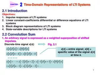
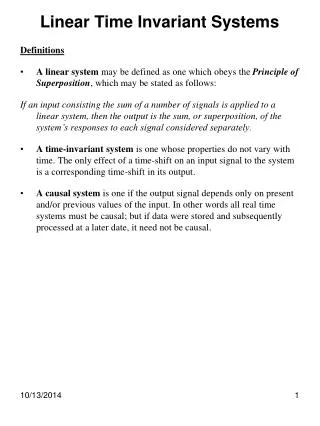
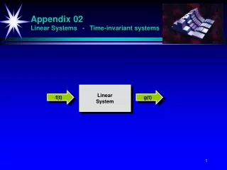
Introduction • Several methods can be used to describe the relationship between the input and output signals of LTI system. • Focus on system description that relate the output signal to the input signal when both are represented as function of time (time domain). • Impulse response defined as output of LTI system due to a unit impulse signal input applied at time t=0 or n=0. • The impulse response completely characterizes the bahaviour of any LTI system.
The impulse response response of a DT system easily obtained by setting the input equal to impulse, δ[n]. • In CT system, a true impulse signal having zero width and infinite amplitude cannot physically be generated and is usually approximated by a pulse of large amplitude and brief duration. • Thus, the impulse response may be interpreted as the system behaviour in response to high-energy input of extremely brief duration.
Given the impulse response, we determine the output due to an arbitrary input signal by expressing the input as a weighted superposition of time-shifted impulses. • By linearity and time invariance, the output signal must be a weighted superposition of time shifted impulse responses. • This weighted superposition is termed the convolution sum for DT system and convolution integral for CT system.
The second method we shall examine for characterizing the input-output behaviour of LTI system is linear constant differential and difference equation. • The third representation is the block diagram, which represents the system as an interconnection of three elementary operation: scalar multiplication, addition and either a time shift for DT system or integration for CY system. • All this time domain represntation are equivalent in the sense that identical outputs results from a given input. However each representation relates input to the output in a different manner.
Convolution • A systematic way to find systems respond. • Convolution integral for CT systems.
Exact Excitation Approximate Excitation The Convolution Integral
The Convolution Integral • All the pulses are rectangular and the same width, the only differences between pulses are when they occur and how tall they are. • So the pulse responses all have the same form except the delayed by some amount, to account for time of occurrence, and multiplied by a weighting constant, to account for the height.
The Convolution Integral Approximating the excitation as a pulse train can be expressed mathematically by or
The Convolution Integral Then, invoking linearity, the response to the overall excitation is (approximately) a sum of shifted and scaled unit pulse responses of the form
The Convolution Integral Convolution Integral
A Graphical Illustration of the Convolution Integral The convolution integral is defined by For illustration purposes let the excitation x(t) and the impulse response h(t) be the two functions below.
A Graphical Illustration of the Convolution Integral We can begin to visualize this quantity in the graphs below.
A Graphical Illustration of the Convolution Integral The functional transformation in going from h(t) to h(t - t) is
A Graphical Illustration of the Convolution Integral The convolution value is the area under the product of x(t) and h(t - t). This area depends on what t is. First, as an example, let t = 5. For this choice of t the area under the product is zero. Therefore if then y(5) = 0.
A Graphical Illustration of the Convolution Integral Now let t = 0. Therefore y(0) = 2, the area under the product.
A Graphical Illustration of the Convolution Integral The process of convolving to find y(t) is illustrated below.
CT Convolution Integral Properties Commutativity Associativity Distributivity
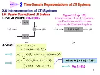
Cascade Connection CT System Interconnections If the output signal from a system is the input signal to a second system the systems are said to be cascade connected. It follows from the associative property of convolution that the impulse response of a cascade connection of LTI systems is the convolution of the individual impulse responses of those systems.
Parallel Connection CT System Interconnections If two systems are excited by the same signal and their responses are added they are said to be parallel connected. It follows from the distributive property of convolution that the impulse response of a parallel connection of LTI systems is the sum of the individual impulse responses.
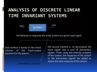
Analysis of Discrete-Time Systems -CONVOLUTION SUM-
System Response • Once the response to a unit impulse is known, the response of any LTI system to any arbitrary excitation can be found • Any arbitrary excitation is simply a sequence of amplitude-scaled and time-shifted impulses • Therefore the response is simply a sequence of amplitude-scaled and time-shifted impulse responses
More Complicated System Response Example System Excitation System Impulse Response System Response
Convolution Sum • A systematic way to find systems response. • Convolution sum for DT systems. • Based on a simple idea, no matter how complicated an excitation signal is, it is simply a sequence of DT impulses. • Therefore, with the assumption that the impulse response to a unit impulse excitation occuring at time n=0 has already found, we will use the convolution technique to find system response.
The Convolution Sum The response y[n] to an arbitrary excitation x[n] is of the form where h[n] is the impulse response. This can be written in a more compact form called the convolution sum.
CT Convolution Sum Properties Convolution is defined mathematically by The following properties can be proven from the definition. Let then and the sum of the impulse strengths in y is the product of the sum of the impulse strengths in x and the sum of the impulse strengths in h.
CT Convolution Sum Properties (continued) Commutativity Associativity Distributivity
CT System Interconnections The cascade connection of two systems can be viewed as a single system whose impulse response is the convolution of the two individual system impulse responses. This is a direct consequence of the associativity property of convolution.
CT System Interconnections The parallel connection of two systems can be viewed as a single system whose impulse response is the sum of the two individual system impulse responses. This is a direct consequence of the distributivity property of convolution.
Relations Between LTI System Properties and the Impulse Response