Download
1 / 25
340 likes | 1.18k Vues
Chapter 3 Time-Domain Analysis of the linear systems. Introduction Stability and Algebraic criteria Analysis of stable error First-order system analysis Second-order system analysis High-order system analysis. Assume:. Zero initial condition; Typical input signal. 3.1 Introduction.

E N D
Chapter 3Time-Domain Analysis of the linear systems • Introduction • Stability and Algebraic criteria • Analysis of stable error • First-order system analysis • Second-order system analysis • High-order system analysis
Assume: Zero initial condition; Typical input signal. 3.1 Introduction 3.1.1 Basic and macroscopically requirements to design a control system. 3.1.2 Basic assumption conditions for analyzing a linear control system The response of a system could be : zero-state zero-input response response transient steady-state portion portion 1) The system must be stable (stability) —First requirement. 2) The control should be accurate (accuracy). 3) The response should be quick-acting (rapidity).
3.1 Introduction 3.1.3 Typical test input signal 1. why to research the test input signal? • The actual input signal of the system is multifarious, normally a standard test input signal should be chosen→to analyze the system performance. • Allow the designer to compare several designs project. • Many input signals of the control systems are similar to the test signals. 2.Which types of the test input signal ? • Step input signal; • Ramp input signal; • Parabolic input signal; • Pulse input signal; • Sinusoidal input signal;
r(t) A 0 t Such as: Such as: switch turn on; relay close train uniformity speed mo-tion; elevator uniformity speed raise. 3.1 Introduction 3. Typical test input signal 2) Ramp input signal 1) Step input signal R(s)=A/s A=1 — unity step input A=1— unity ramp function Application : test signal of the constant-input systems Application : some input-tracking systems
0 ε Unity impulse. Application: some impulse experiments such as: Servo-control system 3.1 Introduction 4) Pulse input signal 3) Parabolic input signal A = 1— unity parabolic signal Application : same as the Ramp signal Such as: Impactive disturbance
Application: Frequency domain analysis of control systems such as:Communication system,Radar system … 3.1 Introduction 5) Sinusoidal signal
3.1 Introduction 3.1.4 Relationship between impulse response and other responses Theorem: 1. For the typical input signals proof: as above :
3.1 Introduction If: g(t) →impulse response of a linear system. g(t) = L-1[ G(s)] h(t) → step response of a linear system. ct(t) → ramp response of a linear system. ctt(t) →parabolic response of a linear system 2. For any signal r(t) we have the Convolution theorem : then: example
A typical unity step response of a control system is shown in following figure 3.1 Introduction 3.1.5The transient performance specifications of a control system • For different system, the research aim is different. For example, the tracking servo control systems are different from the constant-regulating systems. • performance measure — in terms of the step responses of the systems.
Performance specification definition: A Overshoot σ% = 100% B Rise Time tr A Setting time ts B Peak time tp
(for theunder dampedsystems) (for the over damped systems) (for the under damped systems) 3.1 Introduction 1)Rise time tr 2)Peak time tp :
(For the under damped systems) 3.1 Introduction 3)Percent overshoot : 4)Setting time ts : 5)Delay time td : σ% → smoothness of the response. tr、tp、td → rapidity of the response. ts → rapidity of the transient process of the response.
Definition A system work at some original states and is effected by a disturbance (noise) . When the disturbance go off , the system can come back to the original states —— the system is stable. Or else the system is unstable. unstable system is of no practical value) assume: r(t)= δ(t) → R(s)=1 3.2 Stability analysis of the linear systems(Stability: the most important performance for a control system) 3.2.1 What is the Stability of a system ? 3.2.2 The sufficient and necessary conditions of the sta- bility for a linear system.
Conclusion: The sufficient and necessary conditions of the stability for a linear system is: All poles of φ(s) are the poles with negative real part. or : All poles of φ(s) lie in the left-half of the s-plane . 3.2 Stability analysis of the linear systems
Im S-plane Re The sufficient and necessary conditions of the stability for a linear system Graphic representation: Stable region Unstable region The relationship between the system’s stability and the position of poles in S-plane.
R(s) C(s) G(s) - H(s) Assume the polynomial: 3.2 Stability analysis of the linear systems 3.2.3 Routh Criterion Then: for a control system : Characteristic equation of the system: 1+G(s)H (s)=0 Assume :
3.2 Stability analysis of the linear systems We have: we need: all roots of the characteristic equation lie in the left-half of s-plane for a stable system. For the equation : The question is: how could we know the roots all lie in the left-half of s-plane? Routh do it like this:
Tabulate the → Routh table (array): 3.2 Stability analysis of the linear systems
3.2 Stability analysis of the linear systems 1) All elements of the first column of the Routh-table(array) are positive . — The system is and must is stable. conclusion(Routh Criterion): Necessary, sufficient 2) The number of roots with positive real parts is equal to the number of changes in sign of the first column of Routh-table .
3.2 Stability analysis of the linear systems Example 3.2.2 Example 3.2.1 Unstable . 2 roots With positive Real parts Stable
transfer function: Estimate the stability of the system . 3.2 Stability analysis of the linear systems Example 3.2.3 A unity feedback system, Open-loop solution: 0<k<8, the system is stable
3.2 Stability analysis of the linear systems some or other element is equal to zero in the Routh-table. Example 3.2.4 s4 1 1 1 s3 2 2 s2 0 1 s1 ε>0 s0 1 Unstable. 2 roots with positive real parts. Note: Can use a infinitesimalε>0substituting the zero element in the first column.
Example 3.2.5 There are all zero elements in some row of Routh-table. Make auxiliary polynomial : 0 0 multiplied by 1/2 no effect result Unstable,no root in the right-half of s-plane. but there are two pair of roots in the imaginary axis of s-plane:
— unstable, be short of the item 3.2 Stability analysis of the linear systems The order of the auxiliary polynomial is always even indicating the number of symmetrical root pairs . Note: Solving the auxiliary equation, we have: Two inferences about Routh-criterion 1) The characteristic equation is short of one or more than one items —The system must be unstable . Example : 2) The coefficient of the characteristic equation are different in sign. The system must be unstable. Example : — unstable, The coefficient are different in sign.
3.3 steady-stable error Analysis of the linear system Connection to next part