Understanding Linear Time-Invariant Systems in Signals
140 likes | 382 Vues
Explore linear time-invariant systems' characterization through impulse, frequency response, and transfer function. Learn about discrete-time signals, convolution, and comparison to continuous time. Gain insights into the Fundamental Theorem and practical examples.

Understanding Linear Time-Invariant Systems in Signals
E N D
Presentation Transcript
ELM 314 Linear Systems and Signals Spring 2010 LINEAR TIME-INVARIANT (LTI) SYSTEMS Discrete-Time Convolution Dr. Ziya TELATAR Electronics Engineering Department Ankara University
Linear Time-Invariant System • Any linear time-invariant system (LTI) system, continuous-time or discrete-time, can be uniquely characterized by its • Impulse response: response of system to an impulse • Frequency response: response of system to a complex exponential e j 2 p f for all possible frequencies f • Transfer function: Laplace transform of impulse response • Given one of the three, we can find other two provided that they exist May or may not exist May or may not exist
passband Example Frequency Response • System response to complex exponential e jw for all possible frequencies wwherew = 2 p f • Passes low frequencies, lowpass filter |H(w)| H(w) stopband stopband w w -ws -wp wp ws Phase Response Magnitude Response
The Representation of DT Signals in Terms of Impulses x[n] • A Discrete time signal can be composed as; • We can write shifted, scaled impulses as, • In more compact form; • Sifting property • is nonzero only when n=k 0 -1 1 n -1 0 1 -1 0 1 2 3 -1 0 1
h[n] n 0 1 2 3 Discrete-Time Convolution • Output y[n] for inputx[n] • Any signal can be decomposedinto sum of discrete impulses • Apply linear properties • Apply shift-invariance • Apply change of variables y[n] = h[0] x[n] + h[1] x[n-1] = ( x[n] + x[n-1] ) / 2
x[n] 0.5 Example 0.5h[n] 0.5 h[n] 2 • y[n]=0.5h[n]+2h[n-1] 1 2 3 0 1 2h[n-1] 2 n 1 2 3 0 1 2 3 0 1 2 3 0 y[n] 2.5 2 0.5 1 2 3 0
Comparison to Continuous Time • Continuous-time convolution of x(t) and h(t) • For each value of t, we compute a different (possibly) infinite integral. • Discrete-time definition is the continuous-time definition with integral replaced by summation • LTI system • If we know impulse response and input, we can determine the output • Impulse response uniquely characterizes it
Fundamental Theorem • The Fundamental Theorem of Linear Systems • If one inputs a complex sinusoid into an LTI system, then the output will be a complex sinusoid of the same frequency that has been scaled by the frequency response of the LTI system at that frequency • Scaling may attenuate the signal and shift it in phase • Example in continuous time: see handout G • Example in discrete time. Let x[n] = e j W n,H(W) is the discrete-time Fourier transform of h[n] and is also called the frequency response
Continuous Discrete f(t) y(t) f[n] y[n] Ideal Differentiator
h[n] First-order difference impulse response n Image example • Five-tap discrete-time (scaled) averaging FIR filter with input x[n] and output y[n] Lowpass filter (smooth/blur input signal) Impulse response is {1, 1, 1, 1, 1} • First-order difference FIR filter Highpass filter (sharpensinput signal) Impulse response is {1, -1}
Image Example (Contd.) • From lowpass filter to highpass filter original image blurred image sharpened/blurred image • From highpass to lowpass filter original image sharpened image blurred/sharpened image • Frequencies that are zeroed out can never be recovered (e.g. DC is zeroed out by highpass filter) • Order of two LTI systems in cascade can be switched under the assumption that computations are performed in exact precision
Image Example (Contd.) • Precision • Input is represented as eight-bit numbers [0,255] per image pixel (i.e. fewer than three decimal digits of accuracy) • Filter coeffients represented by one decimal digit each • Intermediate computations (filtering) in double-precision floating-point arithmetic (15-16 decimal digits of accuracy) • Output is represented as eight-bit number [-128, 127](i.e. fewer than three decimal digits)