Frequency-Domain of Control Systems
680 likes | 1.36k Vues
Frequency-Domain of Control Systems . Eng R. L. Nkumbwa Copperbelt University 2010. Its all Stability of Control Systems. Introduction. In practice, the performance of a control system is more realistically measured by its time domain characteristics.

Frequency-Domain of Control Systems
E N D
Presentation Transcript
Frequency-Domain of Control Systems Eng R. L. Nkumbwa Copperbelt University 2010
Its all Stability of Control Systems Eng. R. L. Nkumbwa
Introduction • In practice, the performance of a control system is more realistically measured by its time domain characteristics. • The reason is that the performance of most control systems is judged based on the time response due top certain test signals. • In the previous chapters, we have learnt that the time response of a control system is usually more difficult to determine analytically, especially for higher order systems. Eng. R. L. Nkumbwa
Introduction • In design problems, there are no unified methods of arriving at a designed system that meets the time-domain performancespecifications, such as maximum overshoot, rise time, delay time, settling time and so on. Eng. R. L. Nkumbwa
Introduction • On the other hand, in frequency domain, there is a wealth of graphical methods available that are not limited to low order systems. • It is important to realize that there are correlating relations between frequency domain performance in a linear system, • So the time domain properties of the system can be predicted based on the frequency-domain characteristics. Eng. R. L. Nkumbwa
Example: Gun Positional Control Eng. R. L. Nkumbwa
Why use Frequency-Domain? • With the previous concepts in mind, we can consider the primary motivation for conducting control systems analysis and design in the frequency domain to be convenience and the availability of the existing analytical tools. • Another reason, is that, it presents an alternative point of view to control system problems, which often provides valuable or crucial information in the complex analysis and design of control systems. Eng. R. L. Nkumbwa
Frequency-Domain Analysis • The starting point for frequency-domain analysis of a linear system is its transfer system. Eng. R. L. Nkumbwa
Time & Frequency-Domain Specs. • So, what are time-domain specifications by now? • Ok, what of frequency domain specifications? • What are they? • Lets look at the pictorials views… Eng. R. L. Nkumbwa
Time-Domain Specifications Eng. R. L. Nkumbwa
Frequency-Domain Specifications Eng. R. L. Nkumbwa
Wrap Up… • The frequency response of a system directly tells us the relative magnitude and phase of a system’s output sinusoid if the system input is a sinusoid. • What about output frequency? • If the plant’s transfer function is G (s), the open-loop frequency response is G (jw). Eng. R. L. Nkumbwa
Further Frequency Response • In previous sections of this course we have considered the use of standard test inputs, such as step functions and ramps. • However, we will now consider the steady-state response of a system to a sinusoidal input test signal. Eng. R. L. Nkumbwa
Further Frequency Response • The response of a linear constant-coefficient linear system to a sinusoidal test input is an output sinusoidal signal at the same frequency as the input. • However, the magnitude and phase of the output signal differ from those of the input sinusoidal signal, and the amount of difference is a function of the input frequency. Eng. R. L. Nkumbwa
Further Frequency Response • We will now examine the transfer function G(s) where s = jw and graphically display the complex number G(jw) as w varies. • The Bode plot is one of the most powerful graphical tools for analyzing and designing control systems, and we will also consider polar plots and log magnitude and phase diagrams. Eng. R. L. Nkumbwa
Further Frequency Response • How is this different from Root Locus? • The information we get from frequency response methods is different than what we get from the root locus analysis. • In fact, the two approaches complement each other. • One advantage of the frequency response approach is that we can use data derived from measurements on the physical system without deriving its mathematical model. Eng. R. L. Nkumbwa
Further Frequency Response • What is the Importance of Frequency methods? • They are a powerful technique to design a single- loop feedback control system. • They provide us with a viewpoint in the frequency domain. • It is possible to extend the frequency analysis idea to nonlinear systems (approximate analysis). Eng. R. L. Nkumbwa
Who Developed Frequency Methods? • Bode, Nyquist, Nichols and others, in the 1930s and 1940s. • Existed before root locus methods. Eng. R. L. Nkumbwa
What are the advantages? • We can study a system from physical data and determine the transfer function experimentally. • We can design compensators to meet both steady state and transient response requirements. • We can determine the stability of nonlinear systems using frequency analysis (out of the scope of this lecture). • Frequency response methods allow us to settle ambiguities while drawing a root locus plot. • A system can be designed so that the effects of undesirable noise are negligible. Eng. R. L. Nkumbwa
What are the disadvantages? • Frequency response techniques are not as intuitive as root locus. • Find more cons Eng. R. L. Nkumbwa
Concept of Frequency Response • The frequency response of a system is the steady state response of a system to a sinusoidal input. • Consider the stable, LTI system shown below. Eng. R. L. Nkumbwa
Concept of Frequency Response • The input-output relation is given by: Eng. R. L. Nkumbwa
Concept of Frequency Response Eng. R. L. Nkumbwa
Concept of Frequency Response • Obtaining Magnitude M and Phase Ø Eng. R. L. Nkumbwa
Concept of Frequency Response • For linear systems, M and Ø depend only on the input frequency, w. • So, what are some of the frequency response plots and diagrams? Eng. R. L. Nkumbwa
Frequency Response Plots and Diagrams • There are three frequently used representations of the frequency response: • Nyquist diagram: a plot on the complex plane (G(jw)-plane) where M and Ø are plotted on a single curve, and w becomes a hidden parameter. Eng. R. L. Nkumbwa
Frequency Response Plots and Diagrams • Bode plots: separate plots for M and Ø, with the horizontal axis being w is log scale. • The vertical axis for the M-plot is given by M is decibels (db), that is 20log10(M), and the vertical axis for the Ø -plot is Ø in degrees. Eng. R. L. Nkumbwa
Frequency Response Plots and Diagrams • Log-magnitude versus phase plot which is called the Nichols plot. • Now, let us consider each of the techniques in more detail in the following chapters. Eng. R. L. Nkumbwa
Frequency-Domain Systems • We can plot G(jw) as a function of w in three ways: – Bode Plot. – Nyquist Plot. – Nichols Plot (we may not cover this). Eng. R. L. Nkumbwa
Nyquist Diagram or Analysis • The polar plot, or Nyquist diagram, of a sinusoidal transfer function G(jw) is a plot of the magnitude of G(jw) versus the phase angle of G(jw) on polar coordinates as w is varied from zero to infinity. • Thus, the polar plot is the locus of vectors |G(jw)| LG(jw) as w is varied from zero to infinity. Eng. R. L. Nkumbwa
Nyquist Diagram or Analysis • The projections of G(jw) on the real and imaginary axis are its real and imaginary components. • The Nyquist Stability Criteria is a test for system stability, just like the Routh-Hurwitz test, or the Root-Locus Methodology. Eng. R. L. Nkumbwa
Nyquist Diagram or Analysis • Note that in polar plots, a positive (negative) phase angle is measured counterclockwise (clockwise) from the positive real axis. In the polar plot, it is important to show the frequency graduation of the locus. • Routh-Hurwitz and Root-Locus can tell us where the poles of the system are for particular values of gain. Eng. R. L. Nkumbwa
Nyquist Diagram or Analysis • By altering the gain of the system, we can determine if any of the poles move into the RHsP, and therefore become unstable. • However, the Nyquist Criteria can also give us additional information about a system. • The Nyquist Criteria, can tell us things about the frequency characteristics of the system. Eng. R. L. Nkumbwa
Nyquist Diagram or Analysis • For instance, some systems with constant gain might be stable for low-frequency inputs, but become unstable for high-frequency inputs. • Also, the Nyquist Criteria can tell us things about the phase of the input signals, the time-shift of the system, and other important information. Eng. R. L. Nkumbwa
Nyquist Kuo’s View • Kuo et al (2003) suggests that, the Nyquist criterion is a semi-graphical method that determines the stability of a closed loop system by investigating the properties of the frequency domain plot, the Nygmst plot of L(s) is a plot of L (jw) in the polar coordinates of M [L(jw)] versus Re[L(jw)] as w varies from 0 to ∞. Eng. R. L. Nkumbwa
Nyquist Xavier’s View • While, Xavier et al (2004) narrates that, the Nyquist criterion is based on “Cauchy’s Residue Theorem” of complex variables which is referred to as “Principle of Argument”. Eng. R. L. Nkumbwa
The Argument Principle • If we have a contour, Γ, drawn in one plane (say the complex laplace plane, for instance), we can map that contour into another plane, the F(s) plane, by transforming the contour with the function F(s). • The resultant contour, Γ F(s) will circle the origin point of the F(s) plane N times, where N is equal to the difference between Z and P (the number of zeros and poles of the function F(s), respectively). Eng. R. L. Nkumbwa
Nyquist Criterion • Let us first introduce the most important equation when dealing with the Nyquist criterion: • Where: • N is the number of encirclements of the (-1, 0) point. • Z is the number of zeros of the characteristic equation. • P is the number of poles of the open-loop characteristic equation. Eng. R. L. Nkumbwa
Nyquist Stability Criterion Defined • A feedback control system is stable, if and only if the contour ΓF(s) in the F(s) plane does not encircle the (-1, 0) point when P is 0. • A feedback control system is stable, if and only if the contour ΓF(s) in the F(s) plane encircles the (-1, 0) point a number of times equal to the number of poles of F(s) enclosed by Γ. Eng. R. L. Nkumbwa
Nyquist Stability Criterion Defined • In other words, if P is zero then N must equal zero. Otherwise, N must equal P. Essentially, we are saying that Z must always equal zero, because Z is the number of zeros of the characteristic equation (and therefore the number of poles of the closed-loop transfer function) that are in the right-half of the s plane. Eng. R. L. Nkumbwa
Nyquist Manke’s View • While Manke (1997) outlines that, the Nyquist criterion is used to identify the presence of roots of a characteristic equation of a control system in a specified region of s-plane. • He further adds that although the purpose of using Nyquist criterion is similar to RHC, the approach differs in the following respect: Eng. R. L. Nkumbwa
The open loop transfer G(s) H(s) is considered instead of the closed loop characteristic equation 1 + G(s) H(s) = 0 • Inspection of graphical plots G(s) H(s) enables to get more than YES or NO answer of RHC pertaining to the stability of control systems. Eng. R. L. Nkumbwa
Kuo’s Features of Nyquist Criterion • Kuo also outlines the following as the features that make the Nyquist criterion an attractive alternative for the analysis and design of control systems: • In addition to providing the absolute stability, like the RHC, the NC also gives information on the relative of a stable system and the degree of instability. • The Nyquist plot of G(s) H(s) or of L (s) is very easy to obtain. Eng. R. L. Nkumbwa
Kuo’s Features of Nyquist Criterion • The Nyquist plot of G(s) H(s) gives information on the frequency domain characteristics such as Mr, Wr, BW and others with ease. • The Nyquist plot is useful for systems with pure time delay that cannot be treated with the RHC and are difficult to analyze with root locus method. Eng. R. L. Nkumbwa
Any more worries about freqtool… Eng. R. L. Nkumbwa