Use of Frequency Domain

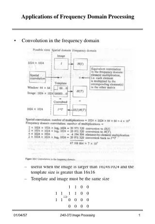
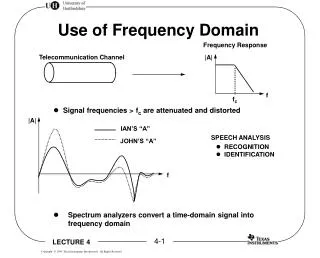
1. Use of Frequency Domain Frequency Response Telecommunication Channel |A| f fc • Signal frequencies > fc are attenuated and distorted |A| IAN’S “A” SPEECH ANALYSIS JOHN’S “A” • RECOGNITION • IDENTIFICATION f • Spectrum analyzers convert a time-domain signal into frequency domain

2. Fourier Series Sum of First 4 Terms of Fourier Series and xp(t) Original Signal xp(t) First 4 Terms of Fourier Series Original xp(t) Tp First 4 Terms of Fourier Series • Periodic signal expressed as infinite sum of sinusoids. • Ck’s are frequency domain amplitude and phase representation • For the given value xp(t) (a square value), the sum of the first four terms of trigonometric Fourier series are: xp(t)  1.0 + sin(t) + sin(3t) + sin(5t)

3. Tp/2 ¥ ò x(t) = åCkej(kw0 t) 1 Ck = x(t) e-j(kw0t) dt Tp k=- ¥ -Tp/2 dw 1 2p Tp TP ¥ ¥ ¥ C(w) dw ò ò x(t) e -jwt dt C(w) = x(t) e-jwt dt 2p dw / 2p - ¥ - ¥ ¥ 1 ò X(w) ejwt dw 2p - ¥ Fourier Transform WHERE w • Increase TP = Period Increases No Repetition = 2p k w0 w • Discrete frequency variable becomes continuous C(w) • Discrete coefficients Ck become continuous FT PAIR normalize = X(w) = x(t) = INVERSE

4. Replace t with Tsn • Continuous x(t) becomes discrete x(n) • Sum rather than integrate all discrete samples Discrete Time Fourier Transform Discrete Time Fourier Transform Fourier Transform Inverse Fourier Transform Inverse Discrete Time Fourier Transform • Limits of integration need not go beyond ±p because the spectrum repeats itself outside ± (every 2) • Keep integration because X(w) is continuous

5. Discrete Fourier Transformation Recall DTFT Pair: • There are an infinite number of time domain samples •  is continuous To Make DTFT Practical: • Take only N time domain samples • Sample the frequency domain, i.e. only evaluate x() at N discrete points. The equal spacing between points is  = 2/N • The result is the Discrete Fourier Transform (DFT) pair:

6. N Samples N Samples 0 Ts 2Ts 3Ts (N-1)Ts 0 1 2 3 N-1  DFT Relationships Time Domain Frequency Domain |x(k)| X(n)   k N-2 N-1 t 0 1 2 N/2 0 n f

7. Practical Considerations • Standard DFT • An example of an 8 point DFT • Writing this out for each value of n • Each term such as requires 8 multiplications • Total number of multiplications required: 8 * 8 = 64Do not forget that each multiplication is complex • 8-point DFT requires 8 2 = 64 multiplications • 1000-point DFT requres 10002 = 1 million multiplications • And all of these need to be summed

8. Fast Fourier Transformation Symmetry Property Periodicity Property Splitting the DFT in two or Manipulating the twiddle factor THE FAST FOURIER TRANSFORM

9. (N/2) 2 Multiplications (N/2) 2 Multiplications Time Savings N/2 Multiplications • For an 8-point FFT, 42 + 42 + 4 = 36 multiplications, saving 64 - 36 = 28 multiplications • For 1000 point FFT, 5002 + 5002 + 500 = 50,500 multiplications, saving 1,000,000 - 50,500 = 945,000 multiplications • Time savings assume 50ns cycle time 8-point FFT saves 1.2 ms • 1000-point FFT saves 47.25ms

10. Splitting the original series into two is called decimation in time • Let us take a short series where N = 8 • Decimate once • Called Radix-2 since we divided by 2 n = {0, 1, 2, 3, 4, 5, 6, 7} n = { 0, 2, 4, 6 } and { 1, 3, 5, 7 } • Decimate again n = { 0, 4 } { 2, 6 } { 1, 5 } and { 3, 7 } Decimation in Time • The result is a savings of N2 – (N/2)log2N multiplications • 1024 point DFT = 1,048,576 multiplications • 1024 point FFT = 5120 multiplication • Decimation simplifies mathematics but there are more twiddle factors to calculate • A practical FFT incorporates these extra factors into the algorithm

11. 3 kn å x(n) W4 X4(k) = 0 1 1 rk rk k å å x(2r) W2 W4 x(2r+1) W2 X4(k) = • Decimate in time into 2 series: + n = {0 , 2} and {1, 3} r=0 r=0 k k k W2 W4 W2 = [ x(0) + x(2) ] + [ x(1) + x(3) ] 2k k 2k W4 W4 W4 = [ x(0) + x(2) ] + [ x(1) + x(3) ] 4-Point FFT • Let us consider an example where N=4: 2p k -j k REMEMBER: WN = e N • We have two twiddle factors. • Can we relate them? 2p 2p -j k -j k 2k 2k * * W2 2 = e = e = W4 4 • Now our FFT becomes:

12. 2k k 2k W4 W4 W4 0 0 0 W4 W4 W4 0 0 0 W4 0 = 0 Flow Diagram • Two DFTs: X4(k) = [ x(0) + x(2) ] + [ x(1) + x(3) ], k=0,1,2,3 • Write out values for k=0 only: X4(0) = [ x(0) + x(2) ] + [ x(1) + x(3) ] • Represent with a flow diagram: X4(0) x(0) x02 x(2) x(1) x13 x(3) • This is only one quarter of the flow diagram

13. 0 0 0 W4 W4 = [ x(0) + x(2) ] + [ x(1) + x(3) ] W4 2p -j 2 1 2 4 * 4 0 W4 W4 W4 = [ x(0) + x(2) ] + [ x(1) + x(3) ] 4 W4 W4 = e = 1 = 0 2 0 W4 W4 W4 = [ x(0) + x(2) ] + [ x(1) + x(3) ] 2p -j 6 * 6 2 4 W4 W4 = e 2 3 2 = -1 = W4 W4 W4 = [ x(0) + x(2) ] + [ x(1) + x(3) ] x(0) 0 0 x(2) 2 1 2 x(1) 0 3 x(3) 2 Full Flow Diagram • Write out all values for k: NOTICE X4(0) X4(1) SPOT THE BUTTERFLY ? X4(2) X4(3)

14. 0 W4 = 1 x1 + k = x2 X1 WN 1 W4 = -j k WN 2 = -1 W4 x1 – k = x2 X2 WN 3 = j W4 x0 X0 0 W4 1 W4 X1 x2 0 W4 0 W4 x1 X2 1 W4 1 W4 x3 X3 The Butterfly Twiddle Conversions Typical Butterfly x1 X1 x2 X2 4 Point FFT Butterfly 4 Point FFT Equations a X0 = (x0 + x2) + (x1+x3) X1 = (x0 – x2) + (x1–x3) X2 = (x0 + x2) – (x1+x3) b X3 = (x0 – x2) – (x1–x3)

15. 2 3 0 1 2 X0=x0+ x2 + x1+x3 = 1 + 0 + 0 + 1 = 2 SAMPLED AT 10kHz X1=x0–x2 + -j(x1–x3) = 1–0 + -j(0–1) = 1 + j Ts= 100 uS X2=(x0+ x2) – (x1+ x3) = (1 + 0) - (0 + 1) = 0 1 X3=(x0–x2)– -j (x1–x3) = (1–0)– -j(0–1) = 1– j NTs A Practical Example Frequency Domain Time Domain Amplitude Amplitude 2 2 Ö2 Ö2 1 1 Frequency Time 0 -5.0 -2.5 0 2.5 5.0 kHz (nTs) 0 3 1 2 FFT Conversion xk = {1,0,0,1} Frequency Spacing F = = AMPLITUDE OF X1= Ö12+j2 = Ö2

16. DSP and FFT • Fast Fourier Transform is a generic name for reducing DFT computations. We considered Radix-2 here, but many other algorithms exist. • The simplified butterflies can be implemented with a DSP very efficiently • Special FFT chips implement it even faster • But DSPs are programmable • And they can perform other operations on the signal • FFT requires address shuffling for faster data table access • Most DSPs can perform shuffling in the background • Modern DSPs can perform an FFT of 1024 samples in well under 5 ms

17. Frequency domain information for a signal is important for processing Sinusoids can be represented by phasors Fourier series can be used to represent any periodic signal Fourier transforms are used to transform signals From time to frequency domain From frequency to time domain DFT allows transform operations on sampled signals DFT computations can be sped up by splitting the original series into two or more series FFT offers considerable savings in computation time DSPs can implement FFT efficiently Summary

18. Sliding Windows

19. Example Frequency Bin New Sample x[0] Old Sample x[N-1] x K2 N Delay K2 = K1N - Note: K1=0.999 Further Frequency Bins + K1 x (X[k]*ej2n/N) K1 x ej2n/N X[k]

20. PHASOR = VECTOR ROTATING Speed = wrad per second Amplitude = A x(t) = Aej(wt) where -1 j = x(t) = a + jb where b f = wt = tan -1 A = a2 + b2 and a The Phasor Model COMPLEX PLANE Im = Imaginary Re = Real Im A b w f Re a 1. Rectangular Form 2. Polar Form ej(wt) = cos(wt) + j sin(wt) w = 2pf p= 180 degrees

21. ej(f ) - e- j(f ) (nwTs + a) f =(w t + a) OR LET THEN sin f = 2j ej(f ) + e- j(f ) AND cos f = 2 j(wt + a ) - j(wt + a ) R (e + e ) x(t) = 2 Modeling Sinusoids REWRITE: ejwt ej(f ) = cos(f ) + jsin(f ) e- j(f ) = cos(f ) - jsin(f ) AS AND Drawing the phasors for cos f Im R/2 In general: b w x(t) = R cos(wt + a ) f A Or as a sum of two phasors: a x(t) = R cos(wt + a ) w -b R/2