The Frequency Domain
The Frequency Domain. Light and the DCT. Pierre-Auguste Renoir: La Moulin de la Galette from http://en.wikipedia.org/wiki/File:Renoir21.jpg. DCT (1D). Discrete cosine transform The strength of the ‘u’ sinusoid is given by C(u) Project f onto the basis function


The Frequency Domain
E N D
Presentation Transcript
The Frequency Domain Light and the DCT Pierre-Auguste Renoir: La Moulin de la Galette from http://en.wikipedia.org/wiki/File:Renoir21.jpg
DCT (1D) • Discrete cosine transform • The strength of the ‘u’ sinusoid is given by C(u) • Project f onto the basis function • All samples of f contribute the coefficient • C(0) is the zero-frequency component – the average value!
DCT (1D) • Consider a digital image such that one row has the following samples • There are 8 samples so N=8 • u is in [0, N-1] or [0, 7] • Must compute 8 DCT coefficients: C(0), C(1), …, C(7) • Start with C(0)
DCT (1D) • Repeating the computation for all u we obtain the following coefficients Spatial domain Frequency domain
DCT (1D) implementation • Since the DCT coefficients are reals, use array of floats • This approach is O(?) public static float[] forwardDCT(float[] data) { final float alpha0 = (float) Math.sqrt(1.0 / data.length); final float alphaN = (float) Math.sqrt(2.0 / data.length); float[] result = new float[data.length]; for (int u = 0; u < result.length; u++) { for (int x = 0; x < data.length; x++) { result[u] += data[x]*(float)Math.cos((2*x+1)*u*Math.PI/(2*data.length)); } result[u] *= (u == 0 ? alpha0 : alphaN); } return result; }
DCT (2D) • The 2D DCT is given below where the definition for alpha is the same as before • For an MxN image there are MxN coefficients • Each image sample contributes to each coefficient • Each (u,v) pair corresponds to a ‘pattern’ or ‘basis function’
DCT basis functions (patterns) Basis functions Basis patterns (imaged functions)
Separability • The DCT is separable • The coefficients can be obtained by computing the 1D coefficients for each row • Using the row-coefficients to compute the coefficients of each column (using the 1D forward transform)
Invertability • The DCT is invertible • Spatial samples can be recovered from the DCT coefficients
Summary of DCT • The DCT provides energy compaction • Low frequency coefficients have larger magnitude (typically) • High frequency coefficients have smaller magnitude (typically) • Most information is compacted into the lower frequency coefficients (those coefficients at the ‘upper-left’) • Compaction can be leveraged for compression • Use the DCT coefficients to store image data but discard a certain percentage of the high-frequency coefficients! • JPEG does this
DCT Compaction and Compression source discarding 95% of dct discarding 99% of dct