Download
1 / 44
450 likes | 553 Vues
This work presented at the Newton Institute in Cambridge discusses the current state and future directions of Quantum Information Theory, particularly focusing on the complexity of local Hamiltonians. Julia Kempe, in collaboration with Oded Regev and Alexei Kitaev, highlights that the 2-local Hamiltonian problem is QMA-complete, and illustrates implications for adiabatic computation and other computational techniques. The presentation explores a bit of history regarding complexity classes such as NP and QMA, providing insights into local Hamiltonians and their applications in quantum computing.

E N D
Newton Institute, Cambridge, August 24th, 2004 Quantum Information Theory: Present Status and Future Directions The Complexity of Local Hamiltonians Julia Kempe CNRS & LRI, Univ. de Paris-Sud, Orsay, France
Also implies: 2-local adiabatic computation is equivalent to standard quantum computation Joint work with Oded Regev and Alexei Kitaev • Result: • 2-local Hamiltonian is QMA complete J. K., Alexei Kitaev and Oded Regev, quant-ph/0406180
Outline • A Bit of History • QMA • Local Hamiltonians • Previous Constructions • The 3-qubit Gadget • Implications • Adiabatic computation • Other applications of the technique
Complexity Theory: • classify “easy” and “hard” A Bit of (ancient) History
“yes” instance: x L V 1 (accept) witness: y “no” instance: x L V 0 (reject) for all “witnesses” y A Bit of (ancient) History • NP – Nondeterministic Polynomial Time: • Def. L NP if there is a poly-time verifier V and • a polynomial p s.t.
0 - false 1 - true 0 = 1, 1 = 0 0 1 1 0 0 0 1 1 “yes” instance: SAT V= (y) 1 (true, accept) witness: y=011000… “no” instance: SAT V= (y) 0 (false, reject) for all “witnesses” y=010110… Example: SAT Formula: • SAT iff there is a satisfying assignment for x1,…,xn (i.e. all clauses true simultaneously).
SAT L L SAT 1 0 1 x y y y=011000… y=010110… V 0 NP complete A languageis NP complete if it is in NP and as hard as any other problem in NP. Cook-Levin Theorem: SAT is NP-complete NP NP-complete x
MAX2SAT is NP-complete MAX2SAT: Input: Formula with 2 variables per clause, number m Output:1(accept) if there is an assignment that violates m clauses 0(reject) all assignments violate >m clauses NP complete 3SAT: 3 variables per clause 3 variables Cook-Levin Theorem: 3SAT is NP-complete 2SAT is in P (there is a poly time algorithm).
witness: | prob 0 (reject) for all “witnesses” | prob 1 (accept) “yes” instance: x Lyes V • QMA – Quantum Merlin Artur = BQNP = “Quantum NP” • Def. L QMA if there is a poly-time quantum verifier V and • a polynomial p s.t. “no” instance: x Lno V QMA 1 (accept) prob 1- 0 (reject) prob 1-
More recent (quantum) History • QMA – Quantum Merlin Artur = BQNP • Def. L QMA if there is a poly-time quantum verifier V and • a polynomial p s.th. • First studied in [Knill’96] and [Kitaev’99] – called it BQNP • “QMA” coined by [Watrous’00] – also: group-nonmembership QMA Kitaev’s quantum Cook-Levin Theorem (’99): Local Hamiltonian is QMA-complete.
Local Hamiltonians • Def. k-local Hamiltonian problem: • Input: k-local Hamiltonian , , Hi acts on k • qubits, a<b constants • Promise: • smallest eigenvalue of H either a or b (b-a const.) • Output: • 1 if H has eigenvalue a • 0 if all eigenvalues of H b
Intuition: Formula: , Hamiltonians: H2 local Hamiltonians H1 Satisfying assignment is groundstate of • Energy-penalty 1 for each unsatisfied constraint. • x1x2 … xn| H |x1x2 … xn = #unsatisfied constraints Local Hamiltonians Penalties for: x1x2x3 = 010 x3x4x5 = 100 …
NP and QMA QMA-completeness? NP-completeness: Verifier V: x1 x2 … y1 y2 … 0 0 … x input 1 witness y … ancilla 0
Verifier Ux : | |0 |0 … |1 H C C H ancilla qubits … • input ? • propagation ancilla |0|1 … |T • output No local way to check! NP and QMA QMA-completeness? NP-completeness: Verifier Vx : y1 y2 … 0 0 … y 1 witness … ancilla 0 3-clauses check: z01 z02 … z03 z04 … zTN z0N z1N z2N t = 0 1 2 3 4 … T
NP and QMA QMA-completeness? NP-completeness: Verifier Vx : Verifier Ux : | |0 |0 … y1 y2 … 0 0 … |1 H C y 1 witness C H … ancilla qubits … ancilla 0 3-clauses check: ||0=|0|1 … |T • input + ? + + + • propagation • output |0 |1 |2 |T | |0|0+|1|1+…+|T|T witness = sum over history
but: • MAX2SAT is NP-complete • 2-local Hamiltonian is NP-hard More recent (quantum) History QMA-completeness: NP-completeness: • log|x|-local Hamiltonian is QMA-compl. • [Kitaev’99] • 5-local Hamiltonian is QMA-compl. • [Kitaev’99] • 3-local Hamiltonian is QMA-compl. • [KempeRegev’02] • 3SAT is NP-complete • 2SAT is in P 2-local Hamiltonian???? Is 2-local Hamiltonian QMA-complete?? • 1-local Hamiltonian is in P
Outline • A Bit of History • QMA • Local Hamiltonians • Previous Constructions • The 3-qubit Gadget • Implications • Adiabatic computation • Other applications of the technique
input Time register {|0, |1,…, |T} Computation qubits • propagation • output Kitaev’s log-local Construction Verifier Ux : |1 | witness = sum over history m N-m T T=poly(N) Local Hamiltonians check: H= Jin Hin + Jprop Hprop + Hout
Kitaev’s log-local Construction Verifier: Ux=UTUT-1…U1 H= Jin Hin + Jprop Hprop + Hout To show: If Ux accepts with prob. 1- on input |,0, then H has eigenvalue . If Ux accepts with prob. on all |,0, then all eigenvalues of H ½-.
|Hprop| =0 |Hout| Completeness Verifier: Ux=UTUT-1…U1 H= Jin Hin + Jprop Hprop + Hout To show: If Ux accepts with prob. 1- on input |,0, then H has eigenvalue . If Ux accepts with prob. on all |,0, then all eigenvalues of H ½-. |Hin| =0
Idea (Kitaev): unary |t | 11…100…0 t T-t |tt| |1010|t,t+1 |tt-1| |110100|t-1,t,t+1 Penalise illegal time states: Sclock - space of legal time-states is preserved (invariant) 5-local Hamiltonians Log-local terms:
Give a high energy penalty to illegal time states to effectively prevent transitions outside Sclock : (|10|t)|Sclock = |tt-1| 3-local Hamiltonians |tt-1| |110100|t-1,t,t+1 5-local terms: Idea [KR’02]: |110100|t-1,t,t+1 |10|t H Sclock
Outline • A Bit of History • QMA • Local Hamiltonians • Previous Constructions • The 3-qubit Gadget • Implications • Adiabatic computation • Other applications of the technique
… Spectrum: H H’ = H + V Energy gap: ||H||>>||V|| 0 groundspace S Three-qubit gadget Idea: use perturbation theory to obtain effective 3-local Hamiltonians from 2-local ones by restricting to subspaces What is the effective Hamiltonian in the lower part of the spectrum?
Case 1: Energy gap>>> ||V|| V--- restriction of V to S V++ - restriction of V to S S S Perturbation Theory Spectrum: H H’ = H + V S Energy gap: ||H||>>||V|| 0 groundspace S What is the effective Hamiltonian in the lower part of the spectrum? Projection Lemma: Heff = V-- (same spectrum) =O(||V||2/)
Case 2: Fine tune the energy gap> ||V|| V--- restriction of V to S V++ - restriction of V to S S S Theorem: Perturbation Theory Spectrum: H H’ = H + V S Energy gap: ||H||>>||V|| 0 groundspace S What is the effective Hamiltonian in the lower part of the spectrum?
First order Third order Second order Perturbation Theory Theorem: H S Energy gap: 0 groundspace S H’ = H + V The lower spectrum of H’ is close to the spectrum of Heff (under certain conditions).
Projection Lemma Perturbation Theory Theorem: First order: ||V||2 << H S Energy gap: 0 groundspace S H’ = H + V The lower eigenvalues (<||V||) of H’ are close to the eigenvalues of Heff (under certain conditions).
2 2 3 3 P2XB P3XC ZZ B C ZZ ZZ A P1XA 1 1 Terms in H’ are 2-local H=P1P2P3 3-local Heff=P1P2P3 3-local Three-qubit gadget
ZZ B C S={|001,|010,|100, |110,|101,|011} =-3 ZZ ZZ Energy gap: A S={|000, |111} 0 Three-qubit gadget H’ = H + V
S V-+ V+- V++ Second order: S S S S V-+ V+- V-- First order: S S Third order: S S Theorem: Three-qubit gadget H’ = H + V 2 3 P2XB P3XC B C S={|001,|010,|100, |110,|101,|011} =-3 Energy gap: A P1XA S={|000, |111} 0 1
|100 Ex.: P1XA P1XA |000 |000 Three-qubit gadget 2 3 P2XB P3XC B C S={|001,|010,|100, |110,|101,|011} =-3 Energy gap: A P1XA S={|000, |111} 0 1 S V-+ V+- Second order: S S Theorem:
P2XB |100 |110 Ex.: P1XA P3XC |000 |111 Three-qubit gadget H’ = H + V 2 3 P2XB P3XC B C S={|001,|010,|100, |110,|101,|011} =-3 Energy gap: A P1XA S={|000, |111} 0 1 V++ S S V-+ V+- Third order: S S Theorem:
Three-qubit gadget 2 3 P2XB P3XC H’ = H + V B C A P1XA 1 Theorem:
Three-qubit gadget 2 3 P2XB P3XC H’ = H + V B C A P1XA 1 Theorem:
Three-qubit gadget 2 3 P2XB P3XC H’ = H + V B C A P1XA 1 Theorem:
H V =-3 -1 Heff 0 0 const. Three-qubit gadget 2 3 P2XB P3XC H’ = H + V B C A P1XA 1 Theorem:
2-local Hamiltonian is QMA-complete • start with the QMA-complete 3-local Hamiltonian • replace each 3-local term by 3-qubit gadget
Outline • A Bit of History • QMA • Local Hamiltonians • Previous Constructions • The 3-qubit Gadget • Implications • Adiabatic computation • Other applications of the technique
Standard quantum circuit: |0…0 |T Adiabatic simulation*: T gates • Hfinal • groundstate • Hinitial • groundstate • |0…0 |0 T’=poly(T): If gap 0(H(t))-1(H(t)) between groundstate and first excited state is 1/poly(T) H(t) = (1-t/T’)Hinitial +t/T’ Hfinal *D. Aharonov, W. van Dam, J. Kempe, Z. Landau, S. Lloyd, O. Regev: "Adiabatic Quantum Computation is Equivalent to Standard Quantum Computation", lanl-report quant-ph/0405098 Implications for Adiabatic Computation • Adiabatic computation [Farhi et al.’00]: • “track” the groundstate of a slowly varying Hamiltonian
adiabat |0…0 |0 Log-local*: H(t) = (1-t/T’) Hin + t/T’ Hprop *D. Aharonov, W. van Dam, J. Kempe, Z. Landau, S. Lloyd, O. Regev: "Adiabatic Quantum Computation is Equivalent to Standard Quantum Computation", lanl-report quant-ph/0405098 Implications for Adiabatic Computation Our result also implies: 2-local adiabatic computation is equivalent to standard quantum computation Replace with 2-local: H(t) = (1-t/T’)(Hin+Jclock Hclock) + t/T’(Hpropgadget+Jclock Hclock)
-2ZA -1P1XA -1P2XA H=P1P2 Heff=P1P2 “Proxy Interaction”: (with A. Landahl) -1Z1ZA -1X2XB -2YAYB Heff=Z1X2 Other applications of the gadget(work in progress) “Interaction at a distance”: H=Z1X2 only XX,YY,ZZ available Useful for Hamiltonian-based quantum architectures
References Quantum Complexity : J. Kempe, A. Kitaev, O. Regev: “The Complexity of the local Hamiltonian Problem”, quant-ph/0406180, to appear in Proc. FSTTCS’04 J. Kempe and O. Regev: "3-Local Hamiltonian is QMA-complete",Quantum Information and Computation, Vol. 3 (3), p.258-64 (2003), lanl-report quant-ph/0302079 Adiabatic Computation : D. Aharonov, W. van Dam, J. Kempe, Z. Landau, S. Lloyd, O. Regev: "Adiabatic Quantum Computationis Equivalent to Standard Quantum Computation", lanl-report quant-ph/0405098, to appear in FOCS’04 *Photo: Oded Regev: Ladybug reading “3-local Hamiltonian” paper
prob 1- prob 0 (reject) prob 1- prob 1 (accept) “yes” instance: x Lyes V MA – Merlin-Artur: Def. L MA if there is a poly-time verifier V and a polynomial p s.t. “no” instance: x Lno V MA 1 (accept) witness: y 0 (reject) for all “witnesses” y