Model quality in L1 prediction error system identification

Model quality in L1 prediction error system identification J-C Carmona LSIS – UMR-CNRS 6168Marseille – France http://www.lsis.org/

Agenda • Introduction • The prediction error framework • Main statistical properties • L1 Final Prediction Error criterion • L1 Akaikes’ Informative Criterion • Distance bound between 2 models • Application & experimental results • Conclusion

1. Introduction • Model Quality: model estimation step : balance ( model error / noise influence) + model validation: - consistency with data : not invalidation - non consistency : invalidation • Validation on “fresh data”: (validation data) - not always possible - validation data are unused in estimation a “poor” estimation Idea: predict the model behaviour from estimation data only: FPE criterion AIC , MDL (Akaike) (Akaike) (Rissanen)

Introduction (2)  Almost ever in L2 prediction error framework !! main advantage: main disadvantages: - L2 optimization simplicity - lack of robustness: “tail-problem” (Rice et al 64) - great statistical sensitivity / data  L1 approach : some interesting recent results - modeling uncertain systems via LP + LSAD criterion (Gustafsson & Mäkilä , Automatica, 96) - FPE criterion in L1 identification (Carmona et al. , CDC02, 02) motivation: prediction residuals rather Laplacian distributed & lack of efficient validation tools in L1 approaches

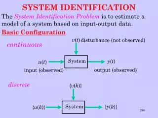
2. The Prediction Error Framework discrete-time SISO system S : parameterized model structure M: one-step ahead predictor : prediction errors : true system S0 :

The Prediction Error Framework (2) estimation data set : estimation criterion : estimation cost function : - L2 approach: LS criterion - L1 approach : LSAD criterion

3. Main Statistical Properties • Convergence properties : ( see L. Ljung 1999) let : where : then : i.e. The estimate converges to « the best approximation » in M

asymptotic properties of the estimate : q0 hyp 1 : Mis globally identifiable at then: , the “true noise” normal distribution : of the estimate around its limit and : with covariance matrix : where : (parameter vector gradient)

asymptotic properties of the estimate (2) Some comments : in L2 case (see L. Ljung 99) , where l0 is the variance of the « true noise ». in L1 case, Q does not depend directly on l0 winteresting in case of noisy measurements zdiserves more investigations !

4. L1 Final Prediction Error criterion Validation criterion principle: = prediction of the (estimation criterion) on estimation data only , i.e. L1 FPE criterion : L2 FPE criterion : noise variance (to be evaluated!)

5. L1 Akaike Information Criterion : Idea: minimization of the information distance model / true system distance: Kullbach-Leibler measure between their PDFs AIC rule: where (L2 case): complexity term: ( MDL criterion ) Rissanen rule :

L1 Akaike Information Criterion (2) L1 case: as for L1 FPE ! : L2 case: 2d/N , versus L1 case: d/N !! first conclusions: - FPE and AIC criteria “exist” in L1 identification - surprise: thy are simpler than in L2 context: weak influence of the noise variance complexity term less penalizing

6. Distance between 2 estimated models New problem: and are two (estimated) models. What about “their distance” ? assumptions: - independent of the estimation method (L2, L1, …) - based on time observations and measurements only : u(t), y(t), e(t), … Assumption: and comes from the same dataZN Based on an original result of L. Ljung and L. Guo (1997)

distance between 2 estimated models (2) past inputs on horizon M: « information » matrix RN : supposed invertible (input PE) hyp: bounded input:  Cu = Max |u(t)| , t  [1,N] Identification problem: extra mode investigation = order increase 1 or 2 i.e. order G2 = order G1 + 1 (or +2) rather « high frequency mode »  tails of impulse response: for k  M, 1k 2k  k 1k- 2k  0 , let: , and: (input periodogram)

distance between 2 estimated models (3) theorem: where: impulse response tails: (assumption 1) L(e j) : linear stable filter correlation term residuals / past inputs: , with: (t) = L(q)[ 1(t) – 2(t) ] ( filtered residuals)

distance between 2 estimated models (3) some comments: 1. Only 1 term: correlation term  simplicity ! 2. Discussion on M / N : in any case N the largest possible !! assumption 1  M large definition : sum of positive terms  M small  trade off !! wehave:

7. Application and experimental results the process • Noise propagating through a semi-infinite duct • Control oriented identification (Active Noise Control) • Not really rational noise spectrum not really rational • OE model structure M : more precisely moles analysis  d = nA

application and experimental results (2) • Comparison FPE criterion L1 / L2 estimation • (use of standard algorithms) . 17 seems to be the best order for both criteria (notice the more marked « knee » in L1 case)

application and experimental results (3) 2. Bound analysis versus model order increase (oder increase of 1 and 2 are presented)

application and experimental results (4) : oder increase = 2 L2 case: odd values L1 case: odd values L1 case: even values L2 case: even values

application and experimental results (5) : some comments L1 estimation: important variations for " low " model orders process dynamics captured step 1 ex: 3  4  5  6 , 9 10 and 11  12  physically confirmed : (5  6)  tHP step 2 ex: 5  7 and 12  14  physically confirmed : (5  7)  1st acoustical mode (12  14)  2d acoustical mode L2 estimation:  same conclusions important variations for " high" model orders Important difference ! Could we conclude: "L1 gives better low order models / L2 gives better high order models " ??

Conclusion • we have shown that: • FPE, AIC rules are " simple” in L1 case  easy to use available (easy to use ) • 2. we have proposed: • a measure of the distance between 2 estimated models • (the cost of the estimation ?!) • 3. Some research "directions " : • - optimization of the choice of M (past inputs horizon) • - analyze the correlation between the terms (L1 case) and (L2 case) • versus • low order model estimates in L1 case / high order in L2 case

Model quality in L1 prediction error system identification