Download
1 / 17
170 likes | 177 Vues
Chemical Thermodynamics 2018/2019. 8 th Lecture: Multicomponent Systems and Chemical Equilibrium Valentim M B Nunes, UD de Engenharia. Introduction.

E N D
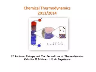
ChemicalThermodynamics2018/2019 8th Lecture: Multicomponent Systems and Chemical Equilibrium Valentim M B Nunes, UD de Engenharia
Introduction Chemical systems evolve spontaneously to minimum G. From now on we can study the chemical equilibrium. To do this we must introduce the thermodynamic treatment of open systems (composition change) The chemical reactions evolves for a dynamic chemical equilibrium characterized for a given equilibrium composition, ξeq, for which: ξis the extent of reaction, 0≤ ξ ≤ 1
Open Systems So far we’ve worked with fundamental equations for closed systems with no composition change. For instance for G we have: If the composition changes Gibbs energy will depend also on the number of moles of each component, so: μi We define μi as the chemical potential of species “i”
Fundamental Equation Considering the definition of chemical potential for a multicomponent system, we can now write: This equation its often mentioned as the Fundamental Equation of Chemical Thermodynamics. It describes open systems (mass can flow in and out, composition can change)
Chemical Equilibrium Consider now p and T constants. We easily obtain: Then, the condition for evolution to equilibrium is: Let us apply this condition to a generic reaction: α A + β B γ C + δ D We define now the extent of reaction, ξ, the units of reaction observed until a given moment. The number of moles or each component it will be: 0 0 for instance for A
Chemical Equilibrium As a consequence we obtain: And: At equilibrium, Generically: Very important result!
Chemical equilibrium in Gaseous Perfect Systems Let us consider now a chemical equilibrium consisting only on ideal gases, that is: α A(g) + β B(g) γ C(g) + δ D(g). In this context signifies a differential coefficient! Remember Then: And, or Q is the reaction quotient
The Equilibrium Constant At equilibrium, ΔGr = 0, and the equilibrium quotient, Qeq is equal to the equilibrium constant, Kp, and then: This is one of the most important equations of chemical thermodynamics as it relates thermodynamic data with the equilibrium constant that can be obtained from the law of mass action. Its very important to note that Kp = Kp(T), that is, the equilibrium constant is a function of temperature only, not a function of total pressure! (what doesn’t mean that the equilibrium composition does not depend on pressure…see next part of lecture!) Recall that all pi values are divided by 1 bar, so Kp is unitless.
Equilibrium Constant in terms of molar fraction and concentration From the Dalton’s law: Then: Δn =(γ + δ) – (α + β) Finally This shows that Ky = Ky(T,p) In terms of concentrations we have from the perfect gas equation of state: Then:
The Effect of pressure in chemical equilibrium Kp is calculated from ΔG0, so, as we mentioned before is independent of pressure. But the equilibrium composition depends on pressure: or As a consequence we can easily obtain: Example: 3 H2(g) + N2(g) 2 NH3(g). In this case Δn < 0, so an increase in pressure will favorite the formation of ammonia. In general an increase in pressure shifts the equilibrium so as to decrease the total number of moles.
Le Chatelier´s Principle What we have just saw for the effect of pressure is a consequence of a more general principle, Le Chatelier’s law: One system in equilibrium that suffers a perturbation will shift spontaneously in order to minimize that perturbation, attaining a new state of equilibrium
Temperature dependence of Kp Recall the Gibbs-Helmholtz equation: or But, Then, And finally we obtain: This is the van’t Hoff Equation It shows that Kp = Kp(T) If a reaction is exothermic, ΔHº<0, then Kp decreases it temperature increase. If the reaction is endothermic then Kp increases with temperature Le Chatelier Principle for temperature!
Temperature dependence of Kp We can rearrange the van’t Hoff equation in the following way: If we assume that ΔHº is constant in a given interval of temperatures, then ln Kp is a linear function of 1/T Ln Kp Slope = -ΔHº/R 1/T
Integrated form Knowing Kp at two temperatures we can calculate the ΔHº of reaction: At two temperatures, and assuming that both ΔHº and ΔSº are constant: And finally:
Chemical Equilibrium in Heterogeneous Systems If a product or reagent is a pure solid or liquid it will not appear in the equilibrium constant, but must be used in the ΔGº calculation. Consider the following reaction: α A(s) + β B(g) = γ C(l) + δ D(g) For the solid an liquid in pure states μi(pure,p) ≈ μiº(pure), what means that there are no pressure dependence. Then for ΔG: ΔGº At equilibrium No A and C involved!
The decomposition of limestone CaCO3(s) = CaO(s) + CO2(g) The condition of equilibrium is: μ (CaO,s) + μ (CO2,g) – μ (CaCO3,s) = 0 Assuming that CO2 is an ideal gas: On the other hand, μ (CaO,s) ≈ μº (CaO,s) and μ (CaCO3,s) ≈ μº (CaCO3,s), and then: μº (CaO,s) + μº (CO2,g) – μº (CaCO3,s) + RT ln pCO2 = 0