Download
1 / 53
530 likes | 684 Vues
Data analysis for impulsive signals using interferometers. Peter R. Saulson Syracuse University Spokesperson, LIGO Scientific Collaboration. Rilke on gravitational wave detection. Though we are unaware of our true status, our actions stem from pure relationship.

E N D
Data analysis for impulsive signals using interferometers Peter R. Saulson Syracuse University Spokesperson, LIGO Scientific Collaboration
Rilke on gravitational wave detection Though we are unaware of our true status, our actions stem from pure relationship. Far away, antennas hear antennas and the empty distances transmit … Pure readiness. Oh unheard starry music! Isn’t your sound protected from all static by the ordinary business of our days? from The Sonnets to Orpheus, First Part, number XII by Rainer Maria Rilke, translated by Stephen Mitchell
Outline • Where I come from: LIGO Scientific Collaboration • What we are doing in the search for gravitational waves • How should one go about looking for poorly-modeled burst signals at low SNR? • A survey of the methods we are trying • Our results to date • A glimpse into the future
Note to students: The search with interferometers has a few novel features, but almost all of them have been strongly inspired (if not taken directly) from the search with resonant detectors. Differences are often a matter of degree only. As resonant detector bandwidths grow, even those differences may shrink.
LIGO and GEO • Four interferometers contribute data to LSC analyses: • 4 km and 2 km interferometers at LIGO Hanford Observatory • 4 km interferometer at LIGO Livingston Observatory • GEO600 • N.B.: No GEO data available for S2, but back on air for S3.
Data Runs S1 run: 17 days (August / September 2002) Four detectors operating: LIGO (L1, H1, H2) and GEO600 Triple-LIGO-coincidence (96 hours) We have carried out three Science Runs(S1--S3) interspersed with commissioning. • Four S1 astrophysical searches published (Phys. Rev. D 69, 2004): • Inspiraling neutron stars 122001 • Bursts 102001 • Known pulsar (J1939+2134) with GEO 082004 • Stochastic background 122004
Data Runs S2 run: 59 days (February—April 2003) Four interferometers operating: LIGO (L1, H1, H2) and TAMA300 plus Allegro bar detector at LSU Triple-LIGO-coincidence (318 hours) • Many S2 searches under way • S3 run: • 70 days (October 2003 – January 2004) – Analysis ramping up…
We search for four classes of signals • Chirps “sweeping sinusoids” from compact binary inspirals • Bursts transients, usually without good waveform models • Periodic, or “CW” from pulsars in our galaxy • Stochastic background cosmological background, or superposition of other signals
h “Chirp” waveform Inspiral Gravitational Waves Compact-object binary systems lose energy due to gravitational waves. Waveform traces history. In LIGO frequency band (40-2000 Hz) for a short time just before merging:anywhere from a few minutes to <<1 second, depending on mass. • Waveform is known accurately for objects up to ~3 M๏ • “Post-Newtonian expansion” in powers of (Gm/rc2) is adequate • Use matched filtering.
(whitened)GW Channel + simulated inspiral SNR Coalescence Time Matched filtering:cross-correlation of data with known signalwaveform
Catastrophic events involving solar-mass compact objects can produce transient “bursts” of gravitational radiation in the LIGO frequency band: core-collapse supernovae merging, perturbed, or accreting black holes gamma-ray burst engines cosmic strings others? Precise nature of gravitational-wave burst (GWB) signals typically unknown or poorly modeled. Can’t base such a broad search on having precise waveforms. Search for generic GWBs of duration ~1ms-1s, frequency ~100-4000Hz. Burst Signals possible supernova waveforms T. Zwerger & E. Muller, Astron. Astrophys. 320 209 (1997)
The burst challenge Interpretation: Broadband observations can reveal details of a signal’s waveform, and thus of the dynamics of the source. Detection: If the waveform is known accurately, then we can use the waveform as a matched template to optimally detect the signal. But without knowledge of the waveform, we have neither the optimal ability to detect the signal, nor a good criterion for choosing among many possible sub-optimal ways to look for the signal. The LSC Burst Group has experimented with a variety of Event Trigger Generators to search for signal candidates in LIGO data.
Burst search example:Time-frequency methods One way to search for bursts is by looking for transients in the time-frequency plane. Here, we illustrate the TFCLUSTERS algorithm. Frequency Time • Compute t-f spectrogram, in short-duration time bins. • Threshold on power in a pixel; search for clusters of pixels. • Find coincident clusters in outputs of all interferometers.
Burst detection methods LSC Burst group has used several variations on time-frequency methods. Also, • Time-domain search for statistical change points • Simple time-domain filtering • Matched filtering for special cases where waveform is known • Black hole “ringdowns” • New search for cosmic string cusp and kink events. Test the list of coincident event candidates for coherence between signals from three LIGO interferometers. Coherence test is also the basis of a search for signals associated with times of gamma-ray bursts or other astrophysical events (“triggered search”.)
For analysis we need… • Identification of detector events • Event Trigger Generation and coincidence • Estimation of expected contribution from background • Time shift analysis • Estimation of efficiency • Simulations • Determination of live-time T • Triple-time subject to vetos • Systematic error estimation and propagation • Calibrations, background estimation, efficiency
Data checks Data Quality: Identify data that do not pass quality criteria • Instrumental errors • Band Limited RMS • Glitch rates from channel • Calibration quality Veto Analysis: • Goal: reduce singles rates without hurting sensitivity • Establish correlations • Study eligibility of veto
Veto Analysis • Strategy: Selection of auxiliary channels with glitches that correlate better with burst triggers • Choice among: Interferometer channels, Wavefront Sensors, Optical Levers, environmental sensors (microphones, accelerometers, seismometers, …) • Method: Coincidence analysis and time-lag plots
Event Trigger Generation Data Conditioning: Different ETGs need different kinds of prefiltering for optimal performance. GW Event Trigger Generators: • Search for unusual transient features in the data.
Other pipeline features Simulations: • Use to optimize ETGs • Employ standard waveforms to measure efficiencies of the search Coincidence Analysis: • Time and frequency coincidence • Waveform consistency: perform a fully coherent analysison candidate events
All tuning done in playground dataset We used a playground dataset for all tuning of thresholds, vetoes, simulation methods. The playground data is about 10% of the run’s duration. After tuning, applied the method to the remaining data, from which analysis results are determined.
Coincidences, random coincidences, and efficiency True coincidences at zero lag, and estimate of random coincidences from non-physical time lags. Determination of search efficiency from artificial addition (in software) of trial signals to data. S1 Comparison of S1 and S2
S1 Burst Search Results • Determine detection efficiency of the end-to-end analysis pipeline via signal injection of various morphologies. • Assume a population of such sources uniformly distributed on a sphere around us: establish upper limit on rate of bursts as a function of their strength • Obtain rate vs. strength plots • End result of analysis pipeline: number of triple coincidence events • Use time-shift experiments to establish number of background events • Use Feldman-Cousins to set confidence upper limits on rate of foreground events: • TFCLUSTERS: <1.6 events/day Burst model: Gaussian/Sine gaussian pulses
hrss: natural measureof strength of unmodeled bursts Without a signal model, it isn’t obvious what feature of signal strength is the most useful measure of what we could have seen in a search that yields an upper limit. We have tested search efficiency against a variety of waveforms. A rather waveform independent measure of search sensitivity is the root-sum-square amplitude, hrss:
A look ahead at the S2 burst search Results from S1 published. S2 results are almost done, but most are not quite ready for sharing. In what follows, I’ll share some of the methods used in the S2 search: What they do How well they work Two burst searches under way: • Untriggered search, like S1, but with two innovations: • New ETG, WaveBurst. • Waveform coherence test, the r-statistic • Coherent search near the time of GRB030329.
use wavelets flexible tiling of the TF-plane by using wavelet packets variety of basis waveforms for bursts approximation Haar, Daubechies, Symlet, Biorthogonal, Meyers. use rank statistics calculated for each wavelet scale robust use local T-F coincidence rules works for 2 and more interferometers coincidence at pixel level applied before triggers are produced WaveBurst: search for burstsusing wavelets
linear dyadic d0 d0 d1 d2 d1 d3 d2 d4 a a a. wavelet transform tree b. wavelet transform binary tree Wavelet Transform LP HP time-scale(frequency) spectrograms
accept reject Coincidence no pixels or L<threshold • Given local occupancy P(t,f) in each channel, after coincidence the black pixel occupancy is for example if P=10%, average occupancy after coincidence is 1% • can use various coincidence policies allows customization of the pipeline for specific burst searches.
channel 1 channel 2 channel 3,… wavelet transform, data conditioning rank statistics wavelet transform, data conditioning rank statistics wavelet transform, data conditioning, rank statistics “coincidence” “coincidence” bp bp bp bp IFO3 cluster generation IFO2 cluster generation IFO1 cluster generation • selection of loudest (black) pixels (black pixel probability P~10% - 1.64 GN rms) “coincidence” Analysis pipeline
Cluster Parameters size – number of pixels in the core volume – total number of pixels density – size/volume amplitude – maximum amplitude power - wavelet amplitude/noise rms energy - power x size asymmetry – (#positive - #negative)/size confidence – cluster confidence neighbors – total number of neighbors frequency - core minimal frequency [Hz] band - frequency band of the core [Hz] time - GPS time of the core beginning duration - core duration in time [sec] Wavelet Cluster Analysis cluster halo cluster core positive negative
r-statistic: an End-of-PipelineWaveform Consistency Test Data Conditioning 100Hz High Pass pseudo-adaptive whitening IFO 1 IFO1 events Event Trigger Generators “excess” power or strain GW /Veto single IFO characterization IFO 1 auxiliary channels Glitches in aux chan as vetos Multi-IFO coincidence, clustering (time, frequency) Uninterpreted limit: Calculate background with time shifts, set upper limit on rate Waveform Consistency (r-statistic test) IFO2 events Interpreted limit: Quantify efficiency for certain waveforms (with simulations) Construct upper limit rate vs strength curves IFO3 events IFO=InterFerOmeter
< > = 0 hrss2 Correlation Analysis
? ? ? ? ? ? The r-statistic test • Correlated time-series “point” in same direction • Pearson r statistic: cosine angle between time-series vectors • Note: Insensitive to relative amplitude scale • Don’t know when signals arrive at geographically distinct detectors • Evaluate r over different physical time-lags • Don’t know signal duration • Evaluate r over range of potential signal durations • r is function of two detectors, not three (or more) • Evaluate geometric mean of significance for all detector pairs Reference: Cadonati gr-qc/0407031
Dt = + 10 ms Dt = - 10 ms confidence versus lag 15 Max confidence: CM(t0) = 13.2 at lag = - 0.7 ms 10 confidence 5 0 -10 0 10 lag [ms] r-statistic Test for Waveform Consistency simulated signal, SNR~60, S2 noise For each triple coincidence candidate event produced by the burst pipeline (start time, duration DT) process pairs of interferometers: After Data Conditioning: Partition the trigger in intervals (50% overlap) of duration t = integration window (20, 50, 100 ms). For each interval, time shift up to 10 ms and build an r-statistic series distribution. If the distribution of the r-statistic is inconsistent with the no-correlation hypothesis: find the time shift yielding maximum correlation confidence CM(j) (j=index for the sub-interval)
Some Technical Details... • Aggressive pre-processing: band-limit to • 100-1600 Hz • Remove all predictable content (effective whitening/line removal):train alinear predictor error filterover 10 s of data (1 s before event start), • emphasis on transients, avoid non-stationary, correlated lines. LHO-4km Waveforms are declared “consistent” (event passes the test) if the correlation confidence is above threshold in all three pairs of interferometers. Correlation confidence: G=max(CML1H1 +CML1H2+CMH1H2)/3 b is the threshold: G > b
Efficiency of the S2 burst search • “All time, all sky” search for short (<1 s timescale) bursts • No external triggers! Generate own from observations • Two step analysis • Trigger generation with WaveBurst • r-statistic test on event candidates • Substantial improvement over S1 sensitivity • About x10 due to reduction in interferometer noise • Remainder of improvement from more effective analysis Preliminary
GRB 030329 Detected by HETE-2, Konus-Wind, Helicon/KoronasF Especially close: z = 0.1685; dL=800Mpc (WMap params) Strong evidence for supernova origin of long GRBs. H1, H2 operating before, during, after burst Radiation from a broadband burst at this distance? Exercise analysis Black hole + debris torus g-rays generated by internal or external shocks Relativistic fireball Triggered searches:g-ray bursts & gravitational waves Hypernovae; collapsars; NS/NS, NS/BH, He/BH, WD/BH mergers; AIC; … For more on GRBs: P. Meszaros, Ann. Rev. Astron. Astrophys. 40 (2002)
< > = 0 hrss2 Correlation Analysis
4 3 2 1 5 Event Identification – Simulated Signal Color coding: “Number of variances above mean” Event strength [ES] calculation: Average value of the “optimal” pixels
Analysis Flow Chart External Trigger Data Inject Simulated Signals Adaptive pre - conditioning Correlation detection algorithm Background region Simulations Signal region Noise event Spectrum Largest event Candidates Efficiency Measurements Upper limits Threshold Threshold
Optimal integration Integration length [ 4-120 ms, uneven steps ] Noise examples Optimal integration Time [ ~ms ] “Huge” Sine-Gaussian F = 361Hz, Q = 8.9 hRSS ~ 6x10-20 [1/Hz] “Small” Sine-Gaussian F = 361Hz, Q = 8.9 hRSS ~ 3x10-21 [1/ Hz] (~ detection threshold) Sensitivity Determination
Dt in [-5,+5] ms for timing uncertainties T in [4,128] ms for short GW bursts t0 is trigger time Analysis Methodology: Externally Triggered Search • Cross-correlate hH1, hH2 near time GRB trigger time … • Near: t in [-120s,+60s] • … and look for cross correlation exceeding threshold • Signal correlated, noise uncorrelated • Random noise correlations will lead to threshold crossing in fraction a of observations • Higher threshold, less likely false positive • Estimated by analysis on noise away from GRB trigger • Set threshold by tolerable false rate a. • This analysis: a = 10% • Methodology applicable to GW burst search associated with any externally generated trigger (e.g., SN, neutrino burst, etc.) For more see: Mohanty et al. gr-qc/0407057 For other x-corr style analyses cf. L. Finn, S. Mohanty, J. Romano, Phys. Rev. D 60 121101 (1999), P. Astone et al., Phys. Rev. D 66 102002 (2002)
GRB030329preliminary result • No event exceeded analysis threshold • Using simulations an upper limit on the associated gravitational wave strength at the detector at the level of hRSS~6x10-20 Hz-1/2 was set • Radiation from a broadband burst at this distance? EGW > 105M8
A fully coherence-basedburst search in S3? • CorrPower: search algorithm for coherent power estimation • Multiple operational modes: • enhanced r-statistic on pre-selected candidate events • external trigger search similar to GRB030329 • continuous search on the whole dataset (compromising on integration times, online?) • Effective unification of coherent triggered and untriggered • Presently undergoing tests • Efficiency at low false-alarm rate • Computing speed
What is CorrPower? (a+b)2 = a2 + b2 + a•b Pcorr = a•b
Checking our instruments and search pipelines • Calibration lines are always present. • We make online tests of data quality, with human review afterwards. • At several times, we inject fake signals by shaking mirrors, to check that they are properly recovered by search pipelines. • Those hardware injections are supplemented by many additional signals added in software to check efficiency of search pipelines. • We carry out intensive reviews of • search software, and of • complete analysis results.