M AT L AB
M AT L AB. Graphics. Basic Plotting Commands. figure : creates a new figure window plot(x) : plots line graph of x vs index number of array plot(x,y) : plots line graph of x vs y


M AT L AB
E N D
Presentation Transcript
MATLAB Graphics
Basic Plotting Commands • figure : creates a new figure window • plot(x) : plots line graph of x vs index number of array • plot(x,y) : plots line graph of x vs y • plot(x,y,'r--') : plots x vs y with linetype specified in string : 'r' = red, 'g'=green, etc for a limited set of basic colours. '' solid line, ' ' dashed, 'o' circles…see graphics section of helpdesk
>> plot(glon,glat) >> xlabel('Longitude'),ylabel('Latitude') >> title('Flight Track : CW96 960607')
>> plot3(glon,glat,palt,'linewidth',2) >> grid >> xlabel('Longitude'),ylabel('Latitude') >> zlabel('Altitude (m)')
Subplots • subplot(m,n,p) : create a subplot in an array of axes >> subplot(2,3,1); >> subplot(2,3,4); P=2 P=1 P=3 m P=4 n
Contour plots • contour(Z) : plot contours of matrix Z • contour(Z,n) : plot n contours (n = integer) • contour(Z,v) : plot contours at levels specified in vector v • contour(X,Y,Z) : plot contours of matrix Z on grid specified by X and Y • [C,h]=contour(…): returns contour matrix C and vector of handles to to contours, h.
contourf(Z) : plot contours filled with colour • clabel(C,h) : add labels to contours • clabel(C,h,v) : add labels only at contours specified in v • clabel(C,h,'manual') : add labels to contours at locations selected with mouse
>> peaks; Peaks is an example function, useful for demonstrating 3D data, contouring, etc. Figure above is its default output. P=peaks; - return data matrix for replotting…
>> P = peaks; >> contour(P)
>> [C,h]=contour(P); >> clabel(C,h);
>> contourf(P,[-9:0.5:9]); >> colorbar
Pseudocolour plots An alternative to contouring – provides a continuous colour-mapped 2D data field • pcolor(Z) : plot pseudocolour plot of Z • pcolor(X,Y,Z) : plot of Z on grid X,Y • shading faceted | flat | interp: set shading option • faceted : show edge lines (default) • flat : don't show edge lines • interp : colour is linearly interpolated to give smooth variation
>> pcolor(P) >> shading flat >> shading interp Data points are at vertices of grid, colour of facet indicates mean value of vertices. Colours are selected by interpolating data range into a colormap
>> pcolor(P);shading flat >> hold on >> contour(P,[1:9],'k') >> contour(P,[-9:-1],'k--') >> contour(P,[0 0],'k','linewidth',2) >> colorbar
colormaps • Surfaces are coloured by scaling the data range to the current colormap. A colormap applies to a whole figure. • Several predefined colormaps exist ('jet' (the default), 'warm','cool','copper','bone','hsv'). Select one with >> colormap mapname >> colormap('mapname') • The current colormap can be retrieved with >> map=colormap
>> caxis([0 8]) >> colorbar
Colormaps are simply 3-column matrices of arbitrary length (default = 64 rows). Each row contains the [RED GREEN BLUE] components of the colour required, specified on a 01 scale. e.g. >> mymap = [ 0 0 0.1 0 0.1 0.2 0.1 0.2 0.3 . . . . . . ] >> colormap(mymap)
Handle Graphics • MATLAB uses a hierarchical graphics model • Graphics objects organised according to their dependencies: e.g. lines must be plotted on axes, axes must be positioned on figures • Every object has a unique identifier, or handle • Handles are returned by creating function • ax(n)=subplot(3,2,n) • h=plot(x,y) • Handles can be used to identify an object in order to inspect (get) or modify (set) its properties at any time
Object Hierarchy root figure axes UI-control UI-menu UI-contextmenu line light image patch surface rectangle text
Each graphics object has properties that can be modified, e.g. for a line object: colour, width, line style, marker style, stacking order on plot,… • Many properties can be modified via the figure window. Tools available depend upon the version running – greatly expanded in version 7. • More useful to use command line – much faster, and can be included in scripts or functions to automate whole process.
Add/edit text zoom Object select Add arrow & line 3D rotate
Properties of an object with handle H, can be inspected/modified by: >> value = get(H,'propertyname') >> set(H,'propertyname',value) • All property values echoed to screen by: >> get(H) • 3 useful functions: • gcf : get current figure – returns handle of current figure • gca : get current axes – returns handle of current axes • gco : get current object – returns handle of current objectCan use these directly, instead of the handle
Current object is last created (usually), or last object clicked on with mouse. >> pp = get(gca,'position') pp = 0.1300 0.1100 0.7750 0.8150 >> set(gca,'position',pp+[0 0.1 0 -0.1]) The code above first gets the position of the current axes – location of bottom left corner (x0, y0), width (dx) and height (dy) (in normalised units) – then resets the position so that the axes sit 0.1 units higher on the page and decreases their height by 0.1 units.
axis 'position' within the figure: (default units are 'normalized') dy dx x0 Figure's 'position' on screen is [x0 y0 dx dy] (default units are pixels) y0
axis position within the figure: it's 'position' (default units are 'normalized') Figure's default position on the page: it's 'paperposition' (default 'paperunits' are 'centimeters') A4 page
Parameter value pairs • Many basic plotting commands accept parameter-value pairs to specify plotting characteristics: • plot(x,y,'para1',value1,'para2',value2,…) • Commonly used parameters : values • 'linewidth' : in points, numeric (default =0.5) • 'color' : 'r','g','b','c','k','m','y' – basic colours (strings) : [R,G,B] – red, green, blue components. Range from 0 to 1 (0 to 100%), eg [0,0.5,1] • 'marker' : shape of marker/symbol to plot '.' point, 'v' triangle, '^' triangle(up pointing),… • 'markeredgecolor','markerfacecolor' : edge and body colours of plotting symbols • 'markersize' : marker size in points (default = 6)
Adding Text to Figures • Basic axis labels and title can be added via convenient functions: >> xlabel('x-axis label text') >> ylabel('y-axis label text') >> title('title text') • Legends for line or symbol types are added via the legend function: >> legend('line 1 caption','line 2 caption',…) >> legend([h1,h2,…],'caption 1','caption 2',…)
>> subplot(1,2,1) >> plot(theta(eval(sw1_2)),palt(eval(sw1_2)),'r');hold on >> plot(theta(eval(sw1_7)),palt(eval(sw1_7)),'g') >> xlabel('\theta (K)'); ylabel('Altitude (m)')
>> hh(1)=plot(xwsc(eval(sw1_2)),palt(eval(sw1_2)),'r'); >> hold on >> hh(2)=plot(xwsc(eval(sw1_7)),palt(eval(sw1_7)),'g'); >> hh(3)=plot(xwsc(eval(sw1_5)),palt(eval(sw1_5)),'b'); >> xlabel('windspeed (m s^{-1})'); >> set(gca,'yticklabel',[]) >> legend(hh([1 3 2]),'sw2','sw5','sw7')
MATLAB uses a subset of TEX commands for mathematical symbols, greek characters etc. • Text may be added at any location via the commands: >> text(x,y,'text to add') – adds text at the specified location (in data coordinates – locations outside the current axes limits are OK) >> gtext('text to add') – adds text at a location selected with the cursor
Obtaining Values from a Figure • The ginput function returns values from cursor-selected points on a graph. >> [x,y] = ginput(n) – selects n values >> [x,y] = ginput – selects values until 'return' key is pressed NB. ginput works on the current axes, and will return values outside visible axis data range if points outside axis frame are selected.
Printing Figures • At its simplest, the command >> print sends the current figure to the default printer. >> print –fn prints figure number n to the default printer • Under unix, a command line switch may be used to specify a printer: >> print –Pprinter
Printing to Files • A wide variety of file formats are supported for printing; the general form is: >> print –driver –options filename e.g. >> print –dps filenameprint postscript file >> print –dpsc filenameprint colour postscript file >> print –depsc filename print colour encapsulated postscript file
>> print –djpeg filenameprint JPEG file (a BAD file format for almost any figure) >> print –dpng –r200 filename print PNG file at 200dpi. All bit-mapped file formats accept a –rnnn option to specify print resolution (default is 150dpi)
.png .jpg
Saving a MATLAB figure • The functions hgsave and hgload save and load a figure to a .fig file – this contains the complete MATLAb handle graphics description of the figure, which can then be modified at a later date. NB the variables used to create the figure are NOT saved. >> hgsave(gcf,'filename') >> hgload('filename.fig')
Putting it all together… • The following slides show the development of a moderately complex figure from raw data : near-surface aircraft measurements of basic meteorology averaged down to 5km intervals along the flight legs.
>> load /cw96/jun07/jun07_all_5km_means.mat >> who Your variables are: mQ mlat mlon msst mtheta mthetav mu mv mws >> plot(mlon,mlat,'o') >> print -dpng -r100 figures/grid-1-data-points
>> [XX,YY]=meshgrid([-125.2:0.05:-124],[39.9:0.05:40.8]); >> gmws=griddata(mlon,mlat,mws,XX,YY); >> pcolor(XX,YY,gmws); shading flat; >> hbar=colorbar; >> hold on >> h1=plot(mlon,mlat,'ko'); >> print -dpng -r100 figures/grid-2-wind-field
>> gu=griddata(mlon,mlat,mu,XX,YY); >> gv=griddata(mlon,mlat,mv,XX,YY); >> quiver(XX,YY,gu,gv,'k-'); >> set(h1,'markeredgecolor','r','markersize',5) >> print -dpng -r100 figures/grid-3-wind-field-and-vectors
>> set(gca,'linewidth',2,'fontweight','bold') >> xlabel('Longitude'); ylabel('latitude') >> set(hbar,'linewidth',2,'fontweight','bold') >> set(get(hbar,'xlabel'),'string','(m s^{-1})','fontweight','bold') >> xlabel('Longitude'); ylabel('latitude') >> title('CW96 : June 07 : 30m wind field') >> load mendocinopatch.mat >> patch(mendocinopatch(:,1),mendocinopatch(:,2),[0.9 0.9 0.9]) >> print -dpng -r100 figures/grid-4-wind-field-and-vectors-and-coast
% generate movie frames from LEM fields [XX,ZZ]=meshgrid(X,Z(iz)); [YY,ZZ]=meshgrid(Y*0,Z(iz)); ZH=ones([102 102])*Z(3); for n=4:33 data1=Q012D_K3{n}; data2=Q012D_I50{n}(iz,:); surf(X,Y,ZH,data1);shading flat; set(gca,'xticklabel',{},'yticklabel',{},'zticklabel',{}); set(gca,'xlim',[min(X) max(X)],'ylim',[min(Y) max(Y)]) hold on surf(XX,YY,ZZ,data2);shading flat; set(gca,'zlim',[0 max(Z(iz))]) Qframes(n-3)=getframe; % NB first n=4, force frames index to hold off % start at 1 to avoid empty frames End % play movie in matlab axis([0 1 0 1 0 1]) set(gca,'visible','off') movie(Qframes,5) % save movie to AVI file movie2avi(Qframes,'testavi.avi','compression','none')