Footprint Evaluation for Volume Rendering
This paper presents a novel feed-forward approach to volume rendering, known as Splatting. We explore the continuous reconstruction of volume functions, shading, and projection into image space. Key techniques include convolution for pixel value filling, effective footprint function management, and the use of view-dependent footprints. We analyze the impact of kernel functions on image quality and showcase the efficiency and parallelizability of our method compared to conventional ray-casting algorithms. Our findings point towards improved rendering with less computational overhead.

Footprint Evaluation for Volume Rendering
E N D
Presentation Transcript
Footprint Evaluation for Volume Rendering A Feed-forward Approach - a.k.a. Splatting (We ‘used’ to be called Ohio Splatting University (OSU))
Process for volume rendering • Reconstruct the continuous volume function • Shade the continuous function • Project this continuous function into image space • Resample the function to get the image
Feed Backward vs. Feed Forward • Feed Backward Method: Image space algorithm (Ray casting) • Feed Forward: Object space method (Splatting) Backward: ray casting
Feed Backward vs. Feed Forward Feed forward: Splatting Splat!
Fill the holes We need to fill the pixel values between the volume projection samples That is, to fit a continuous function through the discrete Samples We can use convolution to do this
i= - j= - Convolution Convolution: g(x,y) = S Sf(i,j) h (x-i, y-j) weight Relative position Sample value f(i,j) The output is a weighted average of inputs g(x,y)
Convolution (2) Another way of thinking convolution is to deposit each function value to its neighbor pixels f(i,j) the weighting function for the deposit this weighting function is called ‘Kernel’
? Volume Rendering and Convolution • Feed Backward (ray casting) views convolution as generating outputs as a weighted average of inputs. • Feed Forward (splatting) views convolution as generating outputs as inputs distributing energy to outputs. Ray casting Splatting
? 3D Kernel for Splatting Need to know the 3D extent of each voxel, and Then project the extent to the image plane This is called ‘footprint’ x Splatting
g(x,y,z) = S S Sf(i,j,k) h (x-i, y-j, z-k) i j k (i,j,k ranges from - to ) - - Footprint function • Effect [(i,j,k)->(x,y,z)] = f(i,j,k) x h (x-i, y-j, z-k) • Effect [(i,j,k)->(x,y)] = f(i,j,k) x h (x-i, y-j, z-k) dz • = f(i,j,k) h (x-i, y-j, z-k) dz
- - Footprint Function (2) • Effect [(i,j,k)->(x,y)] = f(i,j,k) h (x-i, y-j, z-k) dz If we place f(i,j,k) at the origin Then function weight [(i,j,k)->(x,y)] is h (x, y, z) dz = footprint(x,y) (x,y) (0,0) This footprint function defines how much voxel (i,j,k) will deposit its value to pixel (i+x, j+y) -> f(I,j,k) x footprint(x,y)
Footprint Function (3) Pixel (i+x,j+y) receives f(i,j,k) x footprint(x,y) value deposits (i,j,) The final value of pixel (i+x,j+y) will be a total sum of the contributions from its surrouding voxel projections
footprint (x,y) = h (x, y, z) dz - Footprint Function (4) • Evaluating footprint(x,y) on the fly is too time • Consuming - involves integration of the the • kernel function h(x,y,z) • We can build the footprint table at preprocessing time • The kernel function can be any (depends on the renderer)
Footprint Extent Approximate the 3D kernel (h(x,y,z))extent by a sphere
Footprint Table A popular kernel is a three-dimensional Gaussian As 1D integration of 3D Gaussian is still a 2D Gaussian – we can just skip the Z integration and evaluate the Gaussian function on 2D image space after voxel projection Generic footprint table preprocessing
View-dependent footprint It is possible to transform a sphere kernel into A ellipsoid • The projection of an • ellipsoid is an ellipse • We need to transform the • generic footprint table • to the ellipse
Footprint Value Lookup • For rectilinear meshes, the footprint of each sample is identical except for an image-space offset. • The renderer only needs to calculate footprint function once for each view. • Weight is calculated by table lookup at the footprint function value at each pixel that lies within the footprint’s extend
Visibility • Splatting uses the compositing operator to perform visibility • Either front to back or back to front compositing (different formula) • The problem for simply composite sample’s footprint onto the accumulation buffer sample by sample
Effects of No. of entries of the table • Time versus space tradeoff • If a lot of entries, nearest neighbor works fine • If coarse, interpolate from nearest samples. • For smaller table size, interpolation gives much better results. • Images (figure 2 in the paper).
Effects of Kernel function • The choice of kernel can affect the quality of the image. • Examples of cone, gaussian, sync, and bilinear function.
Conclusion • Different from “existing” algorithms (ray casting) • More efficient (sometimes) • Easy to make parallel