View Selection for Volume Rendering
View Selection for Volume Rendering. Udeepta D. Bordoloi Han-Wei Shen Ohio State University. Outline. Introduction Related work Viewpoint evaluation Entropy and view information Noteworthiness Finding the good view View space partitioning View similarity

View Selection for Volume Rendering
E N D
Presentation Transcript
View Selection for Volume Rendering Udeepta D. Bordoloi Han-Wei Shen Ohio State University
Outline • Introduction • Related work • Viewpoint evaluation • Entropy and view information • Noteworthiness • Finding the good view • View space partitioning • View similarity • View likelihood and stability • Partition • Time varying data • Results and discussion • Conclusion and future work
Introduction • With the faster hardware and better algorithms, volume rendering has become a popular method for visualizing volumetric data • Present a novel view selection method for volume rendering • Improve the effectiveness of visualization • Introduces a measure to evaluate a view based on the amount of information displayed( and not displayed)
Introduction • Assume that dataset is centered at the origin • Camera is looking at the origin from a fixed distance • Set of camera position as viewsphere
Three view-point characteristics with each view • View goodness • More important voxels in the volume are highly visible • View likelihood • The number of other viewpoints on the view sphere which yield a view that is similar to the given view • View stability • The maximal change in view when the camera position is shifted within a small neighborhood (defined by a threshold)
Related work • koenderink and van Doorn ( 1976 ) • Had studied singularities in 2 D projections of smooth bodies • for most view ( called stable views), the topology of the projection does not changes for small changes in the viewpoint • the topological changes b/w viewpoints stored in aspect graph • Node : a region of stable views • Edge : transition from one region to an adjacent one • These regions form a partitions of the view space
Related work • Aspect graph defines the minimal number of views required to represent all the topologically different projections of the object • In volume rendering a similar topology based partitioning can not be constructed • Vazquez et al. ( 2001, 2003 ) • Presented an entropy to find good views of polygonal sceces • Entropy : the projected area of the faces of the geometric models in the scene • Entropy is maximized when all the faces project to an equal area on the screen
Related work • Takahashi et al. ( 2005) • Calculate the view entropy for different isosurfaces and interval volumes • Find a weighted average of the individual components • Weights are assigned using the transfer function opacities • This paper ( 2005 ) • Each voxel in the data is assigned a visual significance • Entropy is maximized when the visibilities of the voxels approach the significance values
Viewpoint Evaluation • Better viewpoint, conveys more information about the dataset • The intensity Y at a pixel D • T(s) : transparency of the material b/w the pixel D and the point s • T(s) : visibility of the location s • Y0 : background intensity • 2nd term : contributions of all the voxels along the viewing ray passing through D • G(s) : emission factor g(s) is scaled by visibility T(s) and defined by the users
Viewpoint Evaluation • Transfer function : users set it to highlight the group of voxels they want to see and make others more transparent • Noteworthiness : capture the importance of the voxel as defined by transfer function
Good view • If voxels with high noteworthiness have high visibilities • If the projection of the volumetric dataset contains a high amount of information
Entropy and View Information • Any information source X which outputs a random sequence of symbols {a0,a1,…,aj-1} • Probabilities of symbols occur p={p0,p1,…,pj-1} • aj with probability • The information with aj is I(aj)= - logpj • Entropy
Entropy and View Information • Two properties of the entropy function • For a given number of symbols J, the maximum entropy occurs for the distribution Peq, where { p0 = p1 =…= pj-1 = 1/j} • Entropy is a concave function ,which implies that the local maximum at, is also the global maximum. ( move away from Peq along a straight line in any direction, the entropy decrease)
Entropy and View Information • For each voxel j ,Wj is noteworthiness • For a given view V, Vj(V) is the visibility of the voxel • Visibility denote the transparency of the material b/w the camera and the voxel • For the view V, visual probability qj
Entropy and View Information • Thus, for any view V, visual probability distribution q= {q0,q1,…,qj-1}, j is the number of voxels in the dataset • The entropy of the view
Entropy and View Information • best view( the view with the highest entropy ) • The best view has the highest information content ( averaged over all voxels) • The visual probability distribution of the voxel is the closest to the equal distribution{ p0 = p1 =…= pj-1 = 1/j}, which implies that the voxel visibilities are closet to being proportional to their noteworthiness • To calculate the view entropy, we need to know the voxel visibilities and the noteworthiness
Noteworthiness • Noteworthiness denotes the significance of the voxel to the visualization • It should be high for voxels which are desired to be seen • Two elements of the noteworthiness • Opacity • Color
Noteworthiness • Constructing a histogram of the data • All voxels are assigned to bins of the histogram according to their value, and each voxel gets a probability from the frequency of its bin • Information ij = -logfj, fj is voxel j’s probability • Wj =αjIj ,αjis its opacity • Ignore opacities are zero or close to zero • Algorithm can be made to suit the goals of any particular visualization situation just by changing the noteworthiness
Finding the good view • The dataset is centered at the origin, and camera is at fixed distance from the origin • View sphere : the set of all possible camera position • The voxel visibilities are calculated for each sample view position • Transparency = voxel visibility • Compute the visibilities at the same locations for all views (at the voxel centers) • Use GPU to calculate the visibilities at the exact voxel centers by rendering the volume slices in a front-to-back manner using a modified shear-warp algorithm
Finding the good view • Implementation • Object-aligned slicing direction is most perpendicular to the viewing plane • Use a floating point p-buffer as the volume slices • The 1st slice has no occlusion, so all the voxels in this slice have their visibilities set to unity • Iterate through the rest of the slices in a front-to-back order • In each loop, calculate the visibilities of a slice based on the data opacities and visibilities of the immediate previous slice • In each iteration • The frame-buffer ( p-buffer ) is cleared and the camera set such that the current slice aligns perfectly with the fram-buffer • The immediate previous slice is rendering with a relative shear, and a fragment program combines its opacities with its visibility values • After all the slices are processed, the entropy for the given view direction is calculated using equations (3) and (4)
Finding the good view • The N highest entropy views might not be the best option • Instead we try to find a set of good views whose view samples are well distributed over the view sphere
View space partitioning • A single view does not give enough information to the user • Best N views : a set of views such that all views in the set provide a complete visual description of the dataset • Find the N views by partitioning the view sphere into N disjoint partitions, and selecting a representative view for each partition
View Similarity • Kullback-Leibler ( KL ) distance • Is a distance function from a “true” probability distribution p to a “target” probability distribution p’ • For discrete probability distributions • P={p0,p1,p2,…,pj-i} • P’={p’0,p’1,p’2,…,p’j-i} • Kl distance
View Similarity • If p’j=0 and pj≠0 , D(p||p’) is undefined • Ds(p,p’) is its symmtric form • But D(p||p’) and Ds(p,p’) do not offer any nice upper-bounds
View Similarity • Jensen-Shannon divergence measure • The distance b/w views V1 and V2 ,with distributions q1 and q2
View Likelihood and Stability • View likelihood of a view : the probability of finding another view anywhere on the view-sphere whose view-distance to V is less than a threshold • High likelihood : the dataset projects a similar image for a large number of views
View Likelihood and Stability • Sometimes it is not the view itself but the change in view that provides important information • Stability : the maximum view-distance b/w a view sample and its neighboring view point
Partitioning • Use JS-divergence to find the similarities b/w all pairs of view samples • Cluster the samples to create a disjoint partitioning of view sphere • The number of desired cluster can be specified by the user • Each partition represents a set of similar views • If the view distance b/w two selected view samples is less then a threshold, use a greedapproach to select the next best sample
Time Varying Data • It should show both the data at each time-step , and also the changes occurring from one frame to the next • Using (4) can yield viewpoints in adjacent time-steps that are far from each other, resulting abrupt jumps of the camera during the animation
Time Varying Data -View Information • Suppose n time-steps {t1,t2,…,tn} • Entropy for time-step ti as H(V,ti) ≡HV(ti) • Assume a Markov sequence model for data i.e. in any time-step ti is dependenton the data of the time-step ti-1, but independentof older time-steps • The information measure for the view ( all time-steps)
Time Varying Data -View Information • For time-step ti, the noteworthiness factor of the jth voxel as Wj(ti|ti-1) = • Where 0<k<1 is the weights of voxel opacities and the change in their opacities • The visibility of the voxel for view V is vj(V,ti) • The conditional visual probability qj(ti|ti-1) is • σ is the normalizing factor as eqn.(3) • The entropy is calculated using eqn.(11) and (13)
Results and Discussion • Using a hardware-based visibility calculation • 128 sample views were used for each dataset • The camera positions were obtained by a regular triangular tessellation of a sphere with the dataset place at its center • Run on 2GHz P4, 8xAGP machine with a GeForce 5600 card • For 128-cube dataset, for 128 views took 310s(2.42s per view) • 128*128*80 tooth dataset Fig.4 and fig.5 • 128-cub vortex dataset Fig.6 • For time-varing data 14 time-steps of the 128-cube vortex data was used and k=0.9, Fig.7(a) blue curveis best cumulative entropy for time-series. • Fig.8 show a good entropy and Fig.9 is a bad score
Conclusion and Future Work • Used the properties of the entropy function to satisfy the intuition that good views show the noteworthy voxels more prominently • The user can set the noteworthiness of the voxel by specifying the transfer function, or by using an importance volume, or combination of both • The algorithm can be used both as an aid for human interaction, and also as an oracle to present multiple good views in less interactive contexts • Furthermore, view sampling methods such as IBR can use the sample similarity information to create a better distribution of samples