Algorithm Architecture for Synthetic Aperture Radar (SAR) Ground Processing
300 likes | 397 Vues
Explore the historical background, technical evolution, and key functions of Synthetic Aperture Radar (SAR) processors. Learn about algorithm innovation in SAR processing, from analog to digital advancements. Discover the role of DEC computers in early SAR image formation systems and the impact on algorithm development.

Algorithm Architecture for Synthetic Aperture Radar (SAR) Ground Processing
E N D
Presentation Transcript
Algorithm Architecture for Synthetic Aperture Radar (SAR) Ground Processing Gary A. Mastin, Ph.D. Lockheed Martin Management & Data Systems Intelligence, Surveillance, and Reconnaissance Systems Litchfield Park, Arizona
Overview • SAR Processors - History • Driving Algorithm Functions - Review • Algorithm Architecture vs. Computer Architecture • Discussion Question
In The Beginning… GEMS Precision Optical Correlator
The Advent of Digital Electronics HIRSADAP
The Benefits of the 1960s Space Program • The advent of Digital Image Processing technology • The problem: • We needed pictures of the moon’s surface for selecting landing sites • If the imaging spacecraft couldn’t return to earth, image capture by film wasn’t possible • Late 1960’s television technology was power hungry, heavy, and bulky, but the pictures were pretty good. (Yes, black & white images are good!!!!) • Size, power, and weight constraints limited what we could launch • We didn’t have the communications bandwidth to broadcast live video to the earth from the spacecraft
The Benefits of the 1960s Space Program • The solution: • Send lower-quality cameras into space to meet the size, power, and weight constraints • Characterize the camera deficiencies prior to launch • Turn the video image into a grid of numbers representing intensity onboard the spacecraft. Buffer the data on board, then dump it over the communications link as fast as possible … preferably before crashing into the moon’s surface! • Treat images like large mathematical matrices! Use computers on the ground to correct the camera deficiencies after data receipt. • While we are at it, lets also correct for contrast … and for motion blurs … and for perspective … and, hey, this is pretty powerful stuff!!! • Other applications • Medicine • Defense Synthetic Aperture Radar
Advent of the “Mini-Computer” • The Digital Equipment Corporation (DEC) PDP-series made computing affordable • PDP 8, PDP 10 • PDP 11/45 Big step forward • ~256 KB of core memory • Video terminal for input instead of cards or paper tape • Attached disk, 10s of MB per disk pack (multiple platters) • 800 bpi 9-track tape for archive • RSX 11M operating system supported multiple tasks • Efficient DEC Fortran compiler, assembler, editor, linker, loader… • Interface to peripherals • Video monitors with disk buffers or even core. Dedicated image display functions! • Fixed-point and floating-point FFT hardware • For $250,000 to $750,000, a department or a small company could have its own image processing system.
Video Display Early Digital SAR Image Formation System • Systems like the VAX 11/780 were augmented with peripherals for SAR data input, algorithm processing, and display Phase History Film Digitizer VAX 11/780 System Floating Point Systems AP-120B Array Proc. DCRSI High Density Digital Tape Comtal Digital Image Processor Dunn Camera 1600 bpi 9-Track Tape Vidicon Camera Input Output Processing
-1 RFG_CC RFG_CR c c c r Reference Function Generators DFC Data Format Conversion OFR Output Format Data I/O +1 Forward Inverse CPF Cross-Plane Filter CPF Complex Array Filter IPF In-Plane Filter Fourier Transforms Interpolation Filters CTM DET Corner Turn Magnitude Detect SAR Processing Algorithms • With the flexibility of programming in compiled languages came algorithm innovation “Simple” Matter of Programming • Nomenclature
Key SAR Processing Functions • Dechirp and Range Deskew Dechirp Reference Near Range Receive Pulse Instantaneous Transmit Freq. Tp Far Range Receive Pulse Time fc B t = 0 Scene Center Receive Pulse Transmit Pulse BeforeDechirp A/D Interval After Dechirp 2Ra/c –Dr/c Tp 2Dr/c Freq. After Dechirp Near Range Return BIF Time Center Range Return Adapted from Spotlight Synthetic Aperture Radar: Signal Processing Algorithms By W. Carrara, R. Goodman, R. Majewski, Artech House, 1995. Skew Far Range Return
Key SAR Processing Functions Fourier Reflectivity Space Collection Surface (Slant Plane) Radial Position Of Annulus Determined by Radar Center Frequency Annular Extent Of Data Annulus Determined by Collection Time Length of Annulus Determined by Radar Bandwidth Radar Depression Angle That Determines the Slant Plane Adapted from Spotlight Synthetic Aperture Radar: A Signal Processing Approach by Jakowatz, Wahl, Eichel, Ghiglia, and Thompson
Key SAR Processing Functions • Polar Format Processing (Polar Reformatting) Range Frequency Direction Azimuth Frequency Direction Input Sample Output Sample
Key SAR Processing Functions • 2-D FFT Contiguous Addresses “N” samples/vector Contiguous Addresses “M” samples/new vector Direction of 1-D FFT Direction of 1-D FFT Corner Turn (Transpose) “N” New Vectors “M” Vectors Time
(R2 + I2) Key SAR Processing Functions • Detect and Intensity Remap Piece-Wise Linear Remap Log 10 Output Intensity Input Intensity
Algorithm vs. Computer Architecture • The algorithm processing requirements USUALLY define the computer • Project/Program Requirements • Time to solution (throughput) • Data acquisition geometries & modes Range of data set sizes • Processing options in the baseline algorithm • Derived Requirements that Define the HW Architecture • Sustained/Peak FLOPS (floating point operations per second) • Main memory size • Processor to memory bandwidth • Memory to memory bandwidth • Disk I/O bandwidth • Processed and Unprocessed data archive size
Algorithm vs. Computer Architecture • Cost and Technology issues force compromises • Can’t store the input and output data totally in main memory • Implies a multiple-ingest approach • Large data management implications • Computation-bound. One CPU can’t handle the load. • Implies parallel processing, special purpose processors, or both • Perhaps exploit mathematical separability to improve efficiency • Further data management implications • I/O-bound • Overlapped processing and I/O? • Parallel I/O streams? • Even greater data management implications • Memory bandwidth-bound. Large corner turns are too slow. • Hardware architecture implications • Again, data management implications
Algorithm vs. Computer Architecture • Data management for the computer architecture is a significant algorithm complexity factor! • I can probably architect a dedicated system for SAR ground processing, but… • I don’t want to have different algorithms for different computer architectures • Is it possible to architect an algorithm for maximum portability? • Lets explore the data management issues, then decide
2 1 8 14 7 13 Algorithm Function 1 Algorithm Function 2 Algorithm Function 3 4 3 10 16 9 15 6 5 12 18 11 17 Algorithm vs. Computer Architecture • Multiple Ingest • First scenario (brute force) • Second (sequential) & Third (parallel) scenarios Algorithm Function 2 Algorithm Function 3 Algorithm Function 1 1 2 3 10 11 1 2 3 5 4 Algorithm Function 2 Algorithm Function 3 Algorithm Function 1 4 5 12 6 13 5 4 1 2 3 Algorithm Function 2 Algorithm Function 3 Algorithm Function 1 8 14 15 7 9 5 4 1 2 3
Algorithm vs. Computer Architecture • Computation - Bound • Mathematical Separability • Some 2-D tasks are performed more efficiently as separable 1-D tasks Range Frequency Direction Azimuth Frequency Direction Input Sample Input Sample Output Sample Output Sample Range Frequency Interpolation Azimuth Frequency Interpolation
Algorithm vs. Computer Architecture • I/O – Bound • Multiple options for overlapping Input, Processing, and Output • Sequential Buffering with Processing • Overlapped I/O and Processing Input Memory Buffer Algorithm Function Output Memory Buffer Input Memory Buffer A Algorithm Function Output Memory Buffer A Input Memory Buffer B Algorithm Function Output Memory Buffer B
PE # PE # A A C D B C D E Block # Block # E F G H B F H G K I I K O J L J M N O M N L P P Start Iteration 1 PE # PE # I D I M A E A E F B N B F N G J Block # Block # K C O C K O J G P M H L D H L P Iteration 2 Iteration 3 Algorithm vs. Computer Architecture • Memory Bandwidth – Bound • Distributed Memory Message Passing Exchange Algorithm Perform a local corner Turn on each block Do I = 1, np-1 myswap = XOR(me,I) Send block “myswap” on PE “me” to PE “myswap” Receive block “myswap” on PE “me” from PE “myswap” END DO
Discussion Question • If I want to execute mathematically the same algorithm on the Network Computers that is executed on the Production Computer…. • And if I want to minimize the number of software implementations of the algorithm for cost savings… • Then how should I design my algorithm architecture? Network Computer #1 SGI/Cray J90 64-bit Word 8 Processors Shared Memory Vector Processor Production Computer Archive Product Distribution Fiber Optic Wide-Area Network Network Computer #4 SGI Origin 3000 32-bit Word 128 Processors Distributed Memory Message Passing Network Computer #2 IBM Regatta 32-bit Word 16 Processors Shared Memory Network Computer #3 Sun Blade 2000 32-bit Word 1 Processor Shared Memory
Discussion Question • Lets consider the problem in pieces • How will I use memory efficiently if one computer has a native word length of 64 bits and the others have a native word length of 32 bits? • What are the data management issues when the entire input and output data will not fit into main memory? • Consider non-square input phase history • Remember that we are performing mixed-radix 1-D FFTs (2,3,5,7) • What impact does implementation on a distributed-memory message-passing architecture have on memory management? • How will we perform an out-of-core transpose on a shared memory computer … • If the computer has one processor? • If the computer has multiple processors working simultaneously on different parts of the data set (multiple ingest)?
Conclusion • Hopefully, you can see that creating an architecture-independent transportable algorithm is a daunting challenge. • Hopefully, you understand that addressing this problem early can cost a lot of money, but over time could save large amounts of money in software development and maintenance. • Solving this problem can build customer confidence that your software produces exactly the same result regardless of the computing platform.