Download

1 / 14
150 likes | 206 Vues
Introducing the Method of Least Squares for curve fitting and Wiener filters, explaining the Linear Least-Squares Estimation Problem in signal processing. Discussing the use of data windowing and covariance methods.

E N D
ELG5377 Adaptive Signal Processing Lecture 13: Method of Least Squares
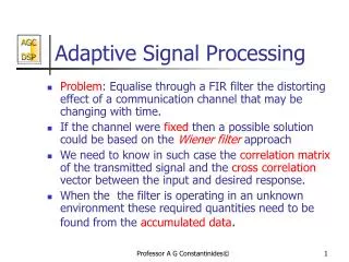
Introduction • Given a sequence of observations x(1), x(2), …, x(N) which occur at time t1, t2, …, tN. • The requirement is to construct a curve that is used to fit these points in some optimum fashion. • Let us denote this curve as f(ti). • The objective is to minimize the squares of the differences between f(ti) and x(i). J = Σ(f(ti)-x(i))2. • The method of least squares can be viewed as an alternative to Wiener filters • Wiener filters are based on ensemble averages • MLS is deterministic in approach and is based on time averages.
Statement of the Linear Least-Squares Estimation Problem • Consider a physical phenomena that is characterized by two sets of variables • d(i) and x(i). • The variable d(i) is observed at time ti in response to the subset of variables x(i), x(i-1), … x(i-M+1). • The response d(i) is modelled by • where wok are unknown parameters of the model and eo(i) represents a measurement error. • The measurement error is an unobservable random variable that is introduced to the model to account for its inaccuracy. (1)
Statement of the Linear Least-Squares Estimation Problem 2 • It is customary to assume that the measurement error is white with 0 mean and variance s2. • The implication of this assumption is that • where the values of x(i), x(i-1), …, x(i-M+1) are all known. • Hence the mean of the response d(i) is uniquely determined by the model.
Statement of the Linear Least-Squares Estimation Problem 3 • The problem we have to solve is to estimate the unknown parameters wok of the multiple linear regression model of (1) given the two observable sets of variables x(i) and d(i) for i= 1, 2, …, N. • To do this we use the linear transversal filter shown below as the model of interest, whose output is y(i) and we use d(i) as the desired response. x(i-1) x(i-M+1) x(i) … e(i) w0* w1* wM-1* y(i) d(i) + + -
Statement of the Linear Least-Squares Estimation Problem 4 Must chose tap weights so as to minimize this cost function
Data Windowing • Typically, we are given data for i= 1 to N, where N > M. • It is only at time M, where d(i) is a function of known data. • Also, for i > N, d(i) has unknown data in its equation. • Covariance method • No assumptions on unknown data, therefore i1 = M and i2 = N. • Autocorrelation method • i1 = 1 and i2 = N+M-1. We assume that x(i) = 0 for i<M and i>N. • Prewindowing and postwindowing. • We will use covariance method.
Orthogonality Principle Revisited 2 • Let e(i) = emin(i) if we select w0, w1, …, wM-1 such that J is minimized. • Then from (2) • The minimum-error time series is orthogonal to the time series x(i-k) applied to tap k of a transversal filter of length M for k = 1, 2, … ,M-1 when the filter is operating in its least-squares condition. • Let ymin(i) be the output of the filter when it is operating in its least squares condition. • d(i) = ymin(i)+emin(i).
Normal Equations and Linear Least-Squares Filters • Let the filter described by the tap weights, w0, w1, …, wM-1 be operating in its least-squares condition. • Therefore k = 0, 1, …, M-1
Normal Equations and Linear Least-Squares Filters: Matrix formulation
Example • x(1)=2, x(2) = 1, x(3) = -0.5, x(4) = 1.2 • d(2) = 0.5, d(3) = 1, d(4) = 0 • Find the two-tap LS filter.