12.3 Correcting for Serial Correlation w/ Strictly Exogenous Regressors
220 likes | 525 Vues
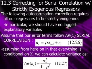
12.3 Correcting for Serial Correlation w/ Strictly Exogenous Regressors. The following autocorrelation correction requires all our regressors to be strictly exogenous -in particular, we should have no lagged explanatory variables Assume that our error terms follow AR(1) SERIAL CORRELATION :.

12.3 Correcting for Serial Correlation w/ Strictly Exogenous Regressors
E N D
Presentation Transcript
12.3 Correcting for Serial Correlation w/ Strictly Exogenous Regressors The following autocorrelation correction requires all our regressors to be strictly exogenous -in particular, we should have no lagged explanatory variables Assume that our error terms follow AR(1) SERIAL CORRELATION : -assuming from here on in that everything is conditional on X, we can calculate variance as:
12.3 Correcting for Serial Correlation w/ Strictly Exogenous Regressors If we consider a single explanatory variable, we can eliminate the correlation in the error term as follows: This provides us with new error terms that are uncorrelated -Note that ytilde and xtilde are called QUASI-DIFFERENCED DATA
12.3 Correcting for Serial Correlation w/ Strictly Exogenous Regressors Note that OLS is not BLUE yet as the initial y1 is undefined -to make OLS blue and ensure the first term’s errors are the same as other terms, we set -note that our first term’s quasi-differenced data is calculated differently than all other terms -note also that this is another example of GLS estimation
12.3 Correcting for Serial Correlation w/ Strictly Exogenous Regressors Given multiple explanatory variables, we have: -note that this GLS estimation is BLUE and will generally differ from OLS -note also that our t and F statistics are now valid and testing can be done
12.3 Correcting for Serial Correlation w/ Strictly Exogenous Regressors Unfortunately, ρ is rarely know, but it can be estimated from the formula: We then use ρhat to estimate: Note that in this FEASIBLE GLS (FGLS), the estimation error in ρhat does not affect FGLS’s estimator’s asymptotic distribution
Feasible GLS Estimation of the AR(1) Model • Regress y on all x’s to obtain residuals uhat • Regress uhatt on uhatt-1 and obtain OLS estimates of ρhat • Use these ρhat estimates to estimate We now have adjusted slope estimates with valid standard errors for testing
12.3 FGLS Notes -Using ρhat is not valid for small sample sizes -This is due to the fact that FGLS is not unbiased, it is only consistent if the data is weakly dependent -while FGLS is not BLUE, it is asymptotically more efficient than OLS (again, large samples) -two examples of FGLS are the COCHRANE-ORCUTT (CO) ESTIMATION and the PRAIS-WINSTEN (PW) ESTIMATION -these estimations are similar and differ only in treating the first observation
12.3 Iterated FGLS -Practically, FGLS is often iterated: -once FGLS is estimated once, its residuals are used to recalculate phat, and FGLS is estimated again -this is generally repeated until phat converges to a number -regression programs can automatically perform this iteration -theoretically, the first iteration satisfies all large sample properties needed for tests -Note: regression programs can also correct for AR(q) using a complicated FGLS
12.3 FGLS vrs. OLS -In certain cases (such as in the presence of unit roots), FGLS can fail to obtain accurate estimates; its estimates can vary greatly from OLS -When FGLS and OLS give similar estimates, FGLS is always preferred if autocorrelation exists -If FGLS and OLS estimates differ greatly, more complicated statistical estimation is needed
12.5 Serial Correlation-Robust Inference -FGLS can fail for a variety of reasons: -explanatory variables are not strictly exogenous -sample size is too low -the form of autocorrelation is unknown and more complicated than AR(1) -in these cases OLS standard errors can be corrected for arbitrary autocorrelation -the estimates themselves aren’t affected, and therefore OLS is inefficient (much like the het-robust correction of simple OLS)
12.5 Autocorrelation-Robust Inference -To correct standard errors for arbitrary autocorrelation, chose an integer g>0 (generally 1-2 in most cases, 1x-2x where x=frequency greater than annually): -where rhat is the residual from regressing x1 on all other x’s and uhat is the residual from the typical OLS estimation
12.5 Autocorrelation-Robust Inference -After obtaining vhat, our standard errors are adjusted using: -note that this transformation is applied to all variables (as any can be listed as x1) -these standard errors are also robust to arbitrary heteroskedasticity -this transformation is done using the OLS subcommand /autcov=1 in SHAZAM, but can also be done step by step:
Serial Correlation-Robust Standard Error for B1hat • Regress y on all x’s to obtain residuals uhat, OLS standard errors, and σhat • Regress x1 on all other x’s and obtain residuals rhat • Use these estimates to estimate vhat as seen previously • Using vhat, obtain new standard errors through:
12.5 SC-Robust Notes -Note that these Serial correlation (SC) robust standard errors are poorly behaved for small sample sizes (even as large as 100) -note that g must be chosen, making this correction less than automatic -if serial correlation is severe, this correction leaves OLS very inefficient, especially in small sample sizes -use this correction only if forced to (some variables not strictly exogenous, lagged dependent variables) -correction is like a hand grenade, not a sniper
12.6 Het in Time Series -Like in cross sectional studies, heteroskedasticity in time series studies doesn’t cause unbiasedness or inconsistency -it does invalidate standard errors and tests -while robust solutions for autocorrelation may correct Het, the opposite is NOT true -Heteroskedasticity-Robust Statistics do NOT correct for autocorrelation -note also that Autocorrelation is often more damaging to a model than Het (depending on the amount of auto (ρ) and amount of Het)
12.6 Testing and Fixing Het in Time Series In order to test for Het: • Serial correlation must be tested for and corrected first • Dynamic Heteroskedasticity (see next section) must not exist Fixing Het is the same as the cross secitonal case: • WLS is BLUE if correctly specified • FGLS is asymptotically valid in large samples • Het-robust corrections are better than nothing (they don’t correct estimates, only s.e.’s)
12.6 Dynamic Het -Time series adds the complication that the variance of the error term may depend on explanatory variables of other periods (and thus errors of other periods) -Engle (1982) suggested the AUTOREGRESSIVE CONDITIONAL HETEROSKEDASTICITY (ARCH) model. A first-order Arch (ARCH(1)) model would look like:
12.6 ARCH -The ARCH(1) model can be rewritten as: -Which is similar to the autoregressive model and has the similar stability condition that α1<1 -While ARCH does not make OLS biased or inconsistent, if it exists a WLS or maximum likelihood (ML) estimation are asymptotically more efficient (better estimates) -note that the usual het-robust standard errors and test statistics are still valid under ARCH
12.6 Het and Autocorrelation…end of the world? -typically, serial correlation is a more serious issue than Het as it affects standard errors and estimation efficiency more -however, a low ρ value may cause Het to be more serious -we’ve already seen that het-robust autocorrelation tests are straightforward
12.6 Het and Autocorrelation…is there hope? If Het and Autocorrelation are found, one can: • Fix autocorrelation using the CO or PW method (Auto command in Shazam) • Apply heteroskedastic-robust standard errors to the regression (Not possible through a simple Shazam command) As a last resort, SC-robust standard errors are also heteroskedastic-robust
12.6 Het and Autocorrelation…is there hope? Alternately, het can be corrected through a combined WLS AR(1) procedure: -Since ut/ht1/2 is homoskedastic, the above equation can be estimated using CO or PW
FGLS with Heteroskedasticity and AR(1) Serial Correlation: • Regress y on all x’s to obtain residuals uhat • Regress log(uhatt2) on all xt’s (or ythat and ythat2) and obtain fitted values, ghatt • Estimate ht: hthat=exp(ghatt) • Estimate the equation By Cochrane-Orcutt (CO) or Prais-Winsten (PW) methods. (This corrects for serial correlation.)