Linear Motion or 1D Kinematics
Linear Motion or 1D Kinematics. With thanks to: Sandrine Colson- Inam , Ph.D. References: Conceptual Physics, Paul G. Hewitt, 10 th edition, Addison Wesley publisher. Outline. The Big Idea Scalars and Vectors Distance versus displacement Speed and Velocity Acceleration

Linear Motion or 1D Kinematics
E N D
Presentation Transcript
Linear Motion or 1D Kinematics With thanks to: Sandrine Colson-Inam, Ph.D References: • Conceptual Physics, Paul G. Hewitt, 10th edition, Addison Wesley publisher
Outline • The Big Idea • Scalars and Vectors • Distance versus displacement • Speed and Velocity • Acceleration • Describing motion with diagrams • Describing motion with graphs • Free Fall and the acceleration of gravity • Describing motion with equations
The Big Idea • Kinematics is the science of describing the motion of objects using words, diagrams, numbers, graphs, and equations. Kinematics is a branch of mechanics. The goal of any study of kinematics is to develop sophisticated mental models which serve to describe (and ultimately, explain) the motion of real-world objects. • Physics is a mathematical science. The underlying concepts and principles have a mathematical basis. Throughout the course of our study of physics, we will encounter a variety of concepts which have a mathematical basis associated with them. While our emphasis will often be upon the conceptual nature of physics, we will give considerable and persistent attention to its mathematical aspect.
Scalars and Vectors • Scalars are quantities which are fully described by a magnitude alone. • Vectors are quantities which are fully described by both a magnitude and a direction. • Check Your Understanding: To test your understanding of this distinction, consider the following quantities listed below. Categorize each quantity as being either a vector or a scalar.
Distance versus Displacement • Distance is a scalar quantity which refers to "how much ground an object has covered" during its motion. • Displacement is a vector quantity which refers to "how far out of place an object is"; it is the object's overall change in position. • To test your understanding of this distinction, consider the motion depicted in the diagram below. A physics teacher walks 4 meters East, 2 meters South, 4 meters West, and finally 2 meters North. • What is the distance covered by the teacher? __________ m • What is his/her displacement? __________ m
Speed versus Velocity • Speed is a scalar quantity which refers to "how fast an object is moving." Speed can be thought of as the rate at which an object covers distance. A fast-moving object has a high speed and covers a relatively large distance in a short amount of time. A slow-moving object has a low speed and covers a relatively small amount of distance in a short amount of time. An object with no movement at all has a zero speed. • Velocity is a vector quantity which refers to "the rate at which an object changes its position."
Average Speed versus Instantaneous Speed • Instantaneous Speed - speed at any given instant in time. • Average Speed - average of all instantaneous speeds; found simply by a distance/time ratio. • You might think of the instantaneous speed as the speed which the speedometer reads at any given instant in time and the average speed as the average of all the speedometer readings during the course of the trip. Since the task of averaging speedometer readings would be quite complicated (and maybe even dangerous), the average speed is more commonly calculated as the distance/time ratio. • Check your understanding: • While on vacation, Lisa Carr traveled a total distance of 440 miles. Her trip took 8 hours. What was her average speed? ________ miles/hr • Now let's consider the motion of that physics teacher again. The physics teacher walks 4 meters East, 2 meters South, 4 meters West, and finally 2 meters North. The entire motion lasted for 24 seconds. Determine the average speed and the average velocity. • Average speed = _______ m/s • Average velocity = _________ m/s in the __________ direction
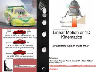
Acceleration • Acceleration is a vector quantity which is defined as the rate at which an object changes its velocity. An object is accelerating if it is changing its velocity. • For objects with a constant acceleration, the distance of travel is directly proportional to the square of the time of travel. • The Direction of the Acceleration Vector • Since acceleration is a vector quantity, it has a direction associated with it. The direction of the acceleration vector depends on two things: • whether the object is speeding up or slowing down • whether the object is moving in the + or - direction • The general RULE OF THUMB is: • If an object is slowing down, then its acceleration is in the opposite direction of its motion.
Check Your Understanding • To test your understanding of the concept of acceleration, consider the following problems and the corresponding solutions. Use the equation for acceleration to determine the acceleration for the following two motions. • Acceleration A = _________ m/s/s or m/s2 • Acceleration B = _________ m/s/s or m/s2
Describing motion with diagrams • Throughout the course, there will be a persistent appeal to your ability to represent physical concepts in a visual manner. • The two most commonly used types of diagrams used to describe the motion of objects are: • ticker tape diagrams • vector diagrams
Ticker Tape Diagrams • A common way of analyzing the motion of objects in physics labs is to perform a ticker tape analysis. A long tape is attached to a moving object and threaded through a device that places a tick upon the tape at regular intervals of time - say every 0.10 second. As the object moves, it drags the tape through the "ticker," thus leaving a trail of dots. The trail of dots provides a history of the object's motion and therefore a representation of the object's motion. • The distance between dots on a ticker tape represents the object's position change during that time interval. A large distance between dots indicates that the object was moving fast during that time interval. A small distance between dots means the object was moving slow during that time interval. Ticker tapes for a fast- and slow-moving object are depicted below. • The analysis of a ticker tape diagram will also reveal if the object is moving with a constant velocity or accelerating. A changing distance between dots indicates a changing velocity and thus an acceleration. A constant distance between dots represents a constant velocity and therefore no acceleration. Ticker tapes for objects moving with a constant velocity and with an accelerated motion are shown below.
Check your understanding • Ticker tape diagrams are sometimes referred to as oil drop diagrams. Imagine a car with a leaky engine that drips oil at a regular rate. As the car travels through town, it would leave a trace of oil on the street. That trace would reveal information about the motion of the car. Renatta Oyle owns such a car and it leaves a signature of Renatta's motion wherever she goes. Analyze the three traces of Renatta's ventures as shown below. Assume Renatta is traveling from left to right. Describe Renatta's motion characteristics during each section of the diagram. 1. 2. 3.
Vector Diagram • Vector diagrams are diagrams which depict the direction and relative magnitude of a vector quantity by a vector arrow. Vector diagrams can be used to describe the velocity of a moving object during its motion. For example, the velocity of a car moving down the road could be represented by a vector diagram. • In a vector diagram, the magnitude of a vector quantity is represented by the size of the vector arrow. If the size of the arrow in each consecutive frame of the vector diagram is the same, then the magnitude of that vector is constant. The diagrams below depict the velocity of a car during its motion. In the top diagram, the size of the velocity vector is constant, so the diagram is depicting a motion of constant velocity. In the bottom diagram, the size of the velocity vector is increasing, so the diagram is depicting a motion with increasing velocity - i.e., an acceleration. • Vector diagrams can be used to represent any vector quantity. In future studies, vector diagrams will be used to represent a variety of physical quantities such as acceleration, force, and momentum. Be familiar with the concept of using a vector arrow to represent the direction and relative size of a quantity. It will become a very important representation of an object's motion as we proceed further in our studies of the physics of motion. • See online animation with varying vector diagrams at http://www.glenbrook.k12.il.us/gbssci/phys/mmedia/kinema/avd.html
Describing motion with graphs • Our study of 1-dimensional kinematics has been concerned with the multiple means by which the motion of objects can be represented. Such means include the use of words, the use of diagrams, the use of numbers, the use of equations, and the use of graphs. • The Importance of Slope • The shapes of the position versus time graphs for these two basic types of motion - constant velocity motion and accelerated motion (i.e., changing velocity) - reveal an important principle. The principle is that the slope of the line on a position-time graph reveals useful information about the velocity of the object. It is often said, "As the slope goes, so goes the velocity."
Position vs. Time Graphs – The meaning of Shape See Animations of Various Motions with Accompanying Graphs Constant Velocity Positive Velocity Changing Velocity Positive Velocity Constant Velocity Slow, Rightward (+) Constant Velocity Fast, Rightward (+) Constant Velocity Fast, Leftward (+) Constant Velocity Slow, Leftward (+) Leftward (-) Velocity Fast to Slow Negative (-) Velocity Slow to Fast
Check Your Understanding • Use the principle of slope to describe the motion of the objects depicted by the two plots below. In your description, be sure to include such information as the direction of the velocity vector (i.e., positive or negative), whether there is a constant velocity or an acceleration, and whether the object is moving slow, fast, from slow to fast or from fast to slow. Be complete in your description.
Position vs. Time Graphs – The meaning of Slope • The slope of the line on a position versus time graph is equal to the velocity of the object. • To determine the slope: • Pick two points on the line and determine their coordinates. • Determine the difference in y-coordinates of these two points (rise). • Determine the difference in x-coordinates for these two points (run). • Divide the difference in y-coordinates by the difference in x-coordinates (rise/run or slope). • Check Your Understanding: Determine the velocity (i.e., slope) of the object as portrayed by the graph below.
Describing Motion with Velocity vs. Time Graphs - Shape • The velocity vs. time graphs for the two types of motion - constant velocity and changing velocity (acceleration) - can be summarized as follows. • The Importance of Slope • The shapes of the velocity vs. time graphs for these two basic types of motion - constant velocity motion and accelerated motion (i.e., changing velocity) - reveal an important principle. The principle is that the slope of the line on a velocity-time graph reveals useful information about the acceleration of the object. If the acceleration is zero, then the slope is zero (i.e., a horizontal line). If the acceleration is positive, then the slope is positive (i.e., an upward sloping line). If the acceleration is negative, then the slope is negative (i.e., a downward sloping line). This very principle can be extended to any conceivable motion. Positive Velocity Positive Acceleration Positive Velocity Zero Acceleration
See Animations of Various Motions with Accompanying Graphs More about slope
Describing Motion with Velocity vs. Time Graphs - Slope Check Your Understanding • The velocity-time graph for a two-stage rocket is shown below. Use the graph and your understanding of slope calculations to determine the acceleration of the rocket during the listed time intervals. • a. t = 0 - 1 second • b. t = 1 - 4 second • c. t = 4 - 12 second
Determining the Area on a v-t Graph • For velocity vs. time graphs, the area bounded by the line and the axes represents the distance traveled. • The diagram shows three different velocity-time graphs; the shaded regions between the line and the axes represent the distance traveled during the stated time interval. • The method used to find the area under a line on a velocity-time graph depends on whether the section bounded by the line and the axes is a rectangle, a triangle or a trapezoid. Area formulae for each shape are given below.
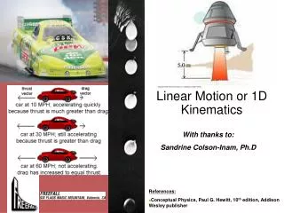
Free Fall and the Acceleration of Gravity • A free-falling object is an object which is falling under the sole influence of gravity. Thus, any object which is moving and being acted upon only by the force of gravity is said to be "in a state of free fall." This definition of free fall leads to two important characteristics about a free-falling object: • Free-falling objects do not encounter air resistance. • All free-falling objects (on Earth) accelerate downwards at a rate of approximately 10 m/s/s (to be exact, 9.8 m/s/s). (acceleration on Earth of 9.8 m/s/s, downward) • This free-fall acceleration can also be demonstrated using a strobe light and a stream of dripping water. If water dripping from a medicine dropper is illuminated with a strobe light and the strobe light is adjusted such that the stream of water is illuminated at a regular rate – say every 0.2 seconds; instead of seeing a stream of water free-falling from the medicine dropper, you will see several consecutive drops. These drops will not be equally spaced apart; instead the spacing increases with the time of fall (as shown in the diagram above), a fact which serves to illustrate the nature of free-fall acceleration.
The Acceleration of Gravity • g = 9.8 m/s/s, downward ( ~ 10 m/s/s, downward) • Thus, velocity changes by 10 m/s every second • If the velocity and time for a free-falling object being dropped from a position of rest were tabulated, then one would note the following pattern. Time (s) Velocity (m/s) 0 0 1 - 9.8 2 - 19.6 3 - 29.4 4 - 39.2 5 - 49.0 Thus tv = gt
Representing Free Fall by Graphs The position vs. time graph for a free-falling object is shown below. • Observe that the line on the graph is curved. A curved line on a position vs. time graph signifies an accelerated motion. Since a free-falling object is undergoing an acceleration of g = 10 m/s/s (approximate value), you would expect that its position-time graph would be curved. A closer look at the position-time graph reveals that the object starts with a small velocity (slow) and finishes with a large velocity (fast). A velocity versus time graph for a free-falling object is shown below. • Observe that the line on the graph is a straight, diagonal line. As learned earlier, a diagonal line on a velocity versus time graph signifies an accelerated motion. Since a free-falling object is undergoing an acceleration (g = 9,8 m/s/s, downward), it would be expected that its velocity-time graph would be diagonal. A further look at the velocity-time graph reveals that the object starts with a zero velocity (as read from the graph) and finishes with a large, negative velocity; that is, the object is moving in the negative direction and speeding up. An object which is moving in the negative direction and speeding up is said to have a negative acceleration (if necessary, review the vector nature of acceleration). Since the slope of any velocity versus time graph is the acceleration of the object (as learned in Lesson 4), the constant, negative slope indicates a constant, negative acceleration. This analysis of the slope on the graph is consistent with the motion of a free-falling object - an object moving with a constant acceleration of 9.8 m/s/s in the downward direction.
How Fast? and How Far? • Free-falling objects are in a state of acceleration. Specifically, they are accelerating at a rate of 10 m/s/s. This is to say that the velocity of a free-falling object is changing by 10 m/s every second. If dropped from a position of rest, the object will be traveling 10 m/s at the end of the first second, 20 m/s at the end of the second second, 30 m/s at the end of the third second, etc. How Fast? • The velocity of a free-falling object which has been dropped from a position of rest is dependent upon the length of time for which it has fallen. The formula for determining the velocity of a falling object after a time of t seconds is: vf = g * t where g is the acceleration of gravity (approximately 10 m/s/s on Earth; its exact value is 9.8 m/s/s). The equation above can be used to calculate the velocity of the object after a given amount of time. How Far? • The distance which a free-falling object has fallen from a position of rest is also dependent upon the time of fall. The distance fallen after a time of t seconds is given by the formula below: d = 0.5 * g * t2 where g is the acceleration of gravity (approximately 10 m/s/s on Earth; its exact value is 9.8 m/s/s). The equation above can be used to calculate the distance traveled by the object after a given amount of time.
The Big Misconception • The acceleration of gravity, g, is the same for all free-falling objects regardless of how long they have been falling, or whether they were initially dropped from rest or thrown up into the air. • BUT "Wouldn't an elephant free-fall faster than a mouse?" NO!! • WHY? • All objects free fall at the same rate of acceleration, regardless of their mass.
Describing Motion with Equations • There are a variety of symbols used in the above equations and each symbol has a specific meaning. • d – the displacement of the object. • t – the time for which the object moved. • a – the acceleration of the object. • vi – the initial velocity of the object. • vf – the final velocity of the object. • Each of the four equations appropriately describes the mathematical relationship between the parameters of an object's motion.
How to use the equations • The process involves the use of a problem-solving strategy which will be used throughout the course. The strategy involves the following steps: • Construct an informative diagram of the physical situation. • Identify and list the given information in variable form. • Identify and list the unknown information in variable form. • Identify and list the equation which will be used to determine unknown information from known information. • Substitute known values into the equation and use appropriate algebraic steps to solve for the unknown information. • Check your answer to insure that it is reasonable and mathematically correct.
Example A Ima Hurryin is approaching a stoplight moving with a velocity of +30.0 m/s. The light turns yellow, and Ima applies the brakes and skids to a stop. If Ima's acceleration is -8.00 m/s2, then determine the displacement of the car during the skidding process. (Note that the direction of the velocity and the acceleration vectors are denoted by a + and a - sign.)
Solution for A • The solution to this problem begins by the construction of an informative diagram of the physical situation. This is shown below. The second step involves the identification and listing of known information in variable form. Note that the vf value can be inferred to be 0 m/s since Ima's car comes to a stop. The initial velocity (vi) of the car is +30.0 m/s since this is the velocity at the beginning of the motion (the skidding motion). And the acceleration (a) of the car is given as - 8.00 m/s2. (Always pay careful attention to the + and - signs for the given quantities.) The next step of the strategy involves the listing of the unknown (or desired) information in variable form. In this case, the problem requests information about the displacement of the car. So d is the unknown quantity. The results of the first three steps are shown in the table below.
Solution for A - end • The next step of the strategy involves identifying a kinematic equation which would allow you to determine the unknown quantity. There are four kinematic equations to choose from. In general, you will always choose the equation which contains the three known and the one unknown variable. In this specific case, the three known variables and the one unknown variable are vf, vi, a, and d. Thus, you will look for an equation which has these four variables listed in it. An inspection of the four equations above reveals that the equation on the top right contains all four variables. • Once the equation is identified and written down, the next step of the strategy involves substituting known values into the equation and using proper algebraic steps to solve for the unknown information. This step is shown below. • (0 m/s)2 = (30.0 m/s)2 + 2*(-8.00 m/s2)*d • 0 m2/s2 = 900 m2/s2 + (-16.0 m/s2)*d • (16.0 m/s2)*d = 900 m2/s2 - 0 m2/s2 • (16.0 m/s2)*d = 900 m2/s2 • d = (900 m2/s2)/ (16.0 m/s2) • d = (900 m2/s2)/ (16.0 m/s2) • d = 56.3 m • The solution above reveals that the car will skid a distance of 56.3 meters. (Note that this value is rounded to the third digit.) • The last step of the problem-solving strategy involves checking the answer to assure that it is both reasonable and accurate. The value seems reasonable enough. It takes a car a considerable distance to skid from 30.0 m/s (approximately 65 mi/hr) to a stop. The calculated distance is approximately one-half a football field, making this a very reasonable skidding distance. Checking for accuracy involves substituting the calculated value back into the equation for displacement and insuring that the left side of the equation is equal to the right side of the equation. Indeed it is! More Practice Problems at http://www.glenbrook.k12.il.us/gbssci/phys/Class/1DKin/U1L6d.html