Download
1 / 11
230 likes | 667 Vues
The Ising Model of Ferromagnetism. by Lukasz Koscielski Chem 444 Fall 2006. Ferromagnetism. Magnetic domains of a material all line up in one direction. In general, domains do not line up no macroscopic magnetization. Can be forced to line up in one direction.

E N D
The Ising Model of Ferromagnetism by Lukasz Koscielski Chem 444 Fall 2006
Ferromagnetism Magnetic domains of a material all line up in one direction In general, domains do not line up no macroscopic magnetization Can be forced to line up in one direction Lowest energy configuration, at low T all spins aligned 2 configurations (up and down) Curie temp - temp at which ferromagnetism disappears Iron: 1043 K Critical point 2nd order phase transition
Models Universality Class – large class of systems whose properties are independent of the dynamic details of the system Ising Model – vectors point UP OR DOWN ONLY simplest Potts Model – vectors point in any direction IN A PLANE Heisenberg Model – vectors point in any direction IN SPACE - binary alloys - binary liquid mixtures - gas-liquid (atoms and vacancies) - superfluid helium - superconducting metals different dimensionality different universality class
Ising Model Low T High T Solved Ising – 1925 1-D Onsager – 1944 2-D Proven computationally intractable - 2000 3-D As T increases, S increases but net magnetization decreases
The 1-D Case The partition function, Z, is given by: With no external magnetic field m = 0. With free boundary conditions Make substitution The 1-D Ising model does NOT have a phase transition.
The 2-D Case The energy is given by For a 2 x 2 lattice there are 24 = 16 configurations Energy, E, is proportional to the length of the boundaries; the more boundaries, the higher (more positive) the energy. In 1-D case, E ~ # of walls In 3-D case, E ~ area of boundary The upper bound on the entropy, S, is kBln3 per unit length. The system wants to minimize F = E – TS. At low T, the lowest energy configuration dominates. At high T, the highest entropy configuration dominates.
Phase Diagrams High T Low T
The 2-D Case - What is Tc? From Onsager: which would lead to negative T so only positive answer is correct kBTc= 2.269J
What happens at Tc? Correlation length – distance over which the effects of a disturbance spread. Approaching from high side of Tc long chain thin film 3D 1D 3D 2D Correlation length increases without bound (diverges) at Tc; becomes comparable to wavelength of light (critical opalescence). Magnetic susceptibility – ratio of induced magnetic moment to applied magnetic field; also diverges at Tc.
Specific heat, C, diverges at Tc. Magnetization, M, is continuous. Entropy, S, is continuous. 2nd Order Phase Transition Magnetization, M, (order parameter) – 1st derivative of free energy – continuous Entropy, S – 1st derivative of free energy – continuous Specific heat, C – 2nd derivative of free energy – discontinuous Magnetic susceptibility, Χ – 2nd derivative of free energy – discontinuous Order parameter, M (magnetization); specific heat, C; and magnetic susceptibility, Χ, near the critical point for the 2D Ising Model where Tc = 2.269.
Critical Exponents Reduced Temperature, t Specific heat Magnetization Magnetic susceptibility Correlation length The exponents display critical point universality (don’t depend on details of the model). This explains the success of the Ising model in providing a quantitative description of real magnets.