Ising Model
Ising Model. Presentation in course Advanced Solid State Physics By Michael He ß. History of critical point behavior. history: three diff periods in the development of the theory of critical point behavior

Ising Model
E N D
Presentation Transcript
Ising Model Presentation in course Advanced Solid State Physics By Michael Heß
History of critical point behavior • history: three diff periods in the development of the theory of critical point behavior • 1. v.d.Waals mean field theory to liquid-gas phase transition but after 1965 numerical calculations and experiments proved that this mean field theory was quantitatively incorrect around the critical point • 2. after 1965 more phenomenological theories based on scaling invariance • 3. same period: another key in critical phenomena theory based on universality (universality: dissimilar systems show similarities near their critical points) • 4. 1971/72: K.Wilson took semi-phenomenological concepts of scaling and universality and converted these ideas into real calculations of critical point behavior
Ernst Ising 10.05.1900 in Köln – 11.05.1998 in Peoria (IL) • Student of Wilhelm Lenz in Hamburg. PhD 1924, • Thesis work on linear chains of coupled magnetic moments. This is known as the Ising model. • The name ‘Ising model’ was coined by Rudolf Peierls in his 1936 publication ‘On Ising’s model of ferromagnetism’. • He survived World War II but it removed him from research. He learned in 1949 (25 years after the publication of his model) that his model had become famous. S. G. Brush, History of the Lenz-Ising Model, Rev. Mod. Phys 39, 883-893 (1962)
Solving of Ising model • invented by W. Lenz and his student E. Ising (1920) • 1D: solved analytically by Ising (1925): no phase transition in 1D and he concluded incorrectly that in higher D also no phase transition • 2D square lattice: solved by L. Onsager (1944), exhibits phase transition • Also in higher dimensions phase transition can be modeled • Istrail showed that computation of the free energy of an arbitrary subgraph based on Ising model will not be approximated computationally intractable (not solvable) by any method for the case 3D and higher - impossible to efficiently compute all possible thermodynamic quantities with arbitrary external fields - it does not mean that the critical exponents or spin-spin correlations cannot be computed near criticality.
1. Critical point and phase transition Critical point of fluid (p=const) 1. temp dependence • Phases for SF6 the curve is • Magnetization for DyAlO3 rho = density Tc = critical temp Fig 1: phase diagram of fluid at p=const Fig 2: Onset of magnetization in ferromagnet
2. Ising model Ising model: • for ferromagnetics invented • Simple Hamiltonian of spins s(r) at lattice point r • Assumptions: - only two states - only nearest neighbor interactions - every pair counts only one time - Hamiltonian: Ising model in 2D Coupling to field pair interaction 3-body interaction s = spins J = energy of interaction (<0 if σi = σj , >0 if σi = -σj ) H = external magnetic field (decreasing H if spins lined up, increasing H if not)
2. Ising model Magnetic interactions: - seek to align spins relative to one another. - spins become effectively "randomized" when thermal energy is greater than the strength of the interaction. - w/o magnetic field the Ising model is symmetric for interchange of ± but magnetic field breaks this symmetry Energy of interaction J: - Jij> 0 the interaction is called ferromagnetic (aligned spins) - Jij< 0 the interaction is called antiferromagnetic (antialigned spins) - Jij= 0 the spins are noninteracting
2. Ising model Thermodynamics of Ising model can be obtained: • for this system, the operation Tr means: • So the free energy is given by • Thermodynamic properties derived by differentiation e.g. average magnetization at site i is derived by δF/ δHi (method of sources)
Ising Model • Free energy functional: • Goal: - model phase changes of real lattices - the 2D square lattice Ising model is simplest model to show phase changes
Ising model in 1D We defined h=H/kT and K=J/kT. The partition function is given by can be calculated exacty. Ising model in 1D: In the following, we will take a look at boundary conditions, thermodynamics and correlations.
Ising model in 1D: Periodic boundaries Periodic boundary conditions are defined by Ising model in 1D with PBC: We assume that there is no external field (h=0). Then, we have We can solve this. Define where i=1…N-1. Then we have Substitution to the partition function gives
Ising model in 1D: Free boundaries Ising model in 1D with free b.c.: Again, we assume that there is no external field (h=0). Then, we have Using the same transformation as before, i.e. where i=1…N-1. We get We have the partition function now. Next, we take a look at free energy and thermodynamics.
Ising model in 1D: Free energy Since we have the partition function, we also have the free energy a) For PBC b) For free b.c. • The difference between boundary conditions becomes negligible at the thermodynamic limit. • The more general way is do this with transfer matrix. Works also for nonzero field. Thermodyn limit
Ising Model • Visualization of Ising model during phase transition http://www.pha.jhu.edu/~javalab/ising/ising.html • Ising model with external field h http://www.physics.uci.edu/~etolleru/IsingApplet/IsingApplet.html
Universality of Ising Model Universality: - the fluctuations close to the phase transition are described by a continuum field with a free energy or Lagrangian as a function of the field values. - Ising model decribes exactly the fluctuations around the critical point In contrast: the mean field doesn’t describe fluctuation at Tc
Applications Magnetism: • In 19th century: two theories: Ampere postulated that permanent magnets are due to permanent internal atomic currents vs. theroy of permanent magnetic moment • Electron spin discovered to describe magnetism • Ising model: investigate if electrons could made to spin in same direction by simple local forces Lattice gas: • Interpret Ising model as a statistical model • B = [0,1],[unoccupied,occupied] B = (σ + 1)/2 σ = [-1,1] • The density of atoms can be controlled by chem pot
Applications Biologie – neurons in brain: • states: firing, not firing • To reproduce average firing rate for each neuron includes activity of each neuron (statistically independent) • To allow for pair interactions when a neuron tends to fire along with another • This energy function only introduces probability biases for a spin having a value and for a pair of spins having the same value. J – NN interaction of firing rate h – self-firing rate