1.7 Turbulent Flow
460 likes | 1.15k Vues
1.7 Turbulent Flow. Turbulent flow is characterized by the random and chaotic motion of fluid molecules. 1.7.1 Time-smoothed variables. Figure 1.7-1 referred steady and unsteady laminar and turbulent flows. The velocity refers to that at a fixed position in the fluid.

1.7 Turbulent Flow
E N D
Presentation Transcript
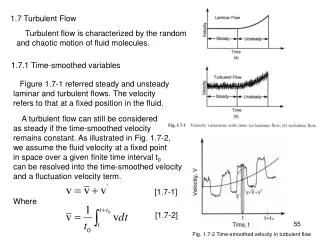
1.7 Turbulent Flow Turbulent flow is characterized by the random and chaotic motion of fluid molecules. 1.7.1 Time-smoothed variables Figure 1.7-1 referred steady and unsteady laminar and turbulent flows. The velocity refers to that at a fixed position in the fluid. A turbulent flow can still be considered as steady if the time-smoothed velocity remains constant. As illustrated in Fig. 1.7-2, we assume the fluid velocity at a fixed point in space over a given finite time interval t0 can be resolved into the time-smoothed velocity and a fluctuation velocity term. [1.7-1] Where [1.7-2] Fig. 1.7-2 Time-smoothed velocity in turbulent flow
The time interval to is small with respect to the time over which v varies but large with respect to the time of turbulent fluctuations. From Eqs. [1.7-1] and [1.7-2], it is obvious that [1.7-3] Since the local pressure is affected by the velocity, we can write a similar expression for the pressure at a fixed point in pace over the same time internal. [1.7-4] The significance of turbulent can be illustrated by fluid flow through a circular pipe. Form Eqs. [1.5-53] and [1.5-54], the expression for laminar flow in a circular pipe is [1.7-5] and [1.7-6]
In contrast for turbulent flow in a circular pipe, it has been proposed and verified experimentally that [1.7-7] And Eq. [1.7-7] is known as the Blasius one-seventh power law. [1.7-8] As shown in Fig. 1.7-3, the velocity distribution is significantly more uniform in the case of turbulent flow, as a result of better mixing in the bulk fluid. 1.7-2 Time-smoothed governing equations Substituting Eqs.[1.7-1] into Eq.[1.3-5] and then taking the time average according to Eqs [1.7-2] and [1.7-3], we obtain [1.7-9] which is the time-smoothed equation of continuity for incompressible fluids.
Similar, substituting Eqs. [1.7-1]and [1.7-4] into [1.5-6] and then taking the time average according to Eqs.[1.7-2] and [1.7-3], we get the following time-smoothed equation of motion [1.7-10] , resulted from turbulent velocity, is sometimes called the Reynolds stresses. [1.7-11] Since the fluid in Ω exerts a stress t.n on its surroundings, the surroundings can be considered to exert a stress –t.n on the fluid in Ω. Note thatτis a tensor (p.36), and t.n is a vector (p.46). The vector t.n is the force exerts on its surrounding, which is due to the viscous force and can be expressed by the velocity components.
1.7.3 Turbulent momentum flux Several semiempirical relations have been proposed for the Reynolds stresses t’, in order to solve Eq. [1.7-10] for velocity distribution in turbulent flow. 1.7.3.1 Eddy viscosity Boussinesq proposed the following form By analogy with Eq.[1.1-2], Newton’s law of visiosity. The coefficient m’ is a turbulent or eddy viscosity and is position-dependent. [1.7-12] 1.7.3.2 Prandtl’s mixing length Prandtl proposed the concept of the mixing length based on the assumption that eddies move about in a fluid like molecules do in a gas. The mixing length plays a role somewhat similar to that of the mean free path in the gas kinetic theory. [1.7-13] and from Eq.[1.7-12] [1.7-14] Where l, called the mixing length, is a function of position, for example l= ay, where y is the distance from the solid surface.
1.8 Momentum transfer correlations 1.8.1 External flow 1.8.1.1 Flow over a flat plate Flow over a flat plate is laminar for local Reynolds number Rez < 2 x 10⁵. The following correlation can be used for laminar flow over a flat plate [1.8-1] where, as shown in Eq. [1.1-6] and [1.8-2] [1.8-3] From these equations the friction coefficient averaged over a distance L from the leading edge of the plate is Substituting Eq. [1.8-1] into q. [1.8-4] [1.8-4] [1.8-5]
Hence where For turbulent flow over a flat plate the following empirical correlation has been suggest and from Eq. [1.8-4] [1.8-6] [1.8-7] [1.8-8] [1.8-9]
1.8.1.2 Flow normal to a cylinder For incompressible flow normal to a cylinder of diameter D, the drag coefficient is a function of Reynolds number, as shown in Fig. 1.8-1(a) [1.8-10] Where, according to Eq. [1.1-37], and Fig. 1.8-1
1.8.1.3 Flow past a sphere The creeping incompressible flow around a sphere of diameter D is [1.8-13] where CD and ReD are defined in Eqs. [1.8-11] and [1.8-12], respectively. The following empirical correlations can be used for higher ReD: [1.8-14] and [1.8-15] The experimental data of Cd as a function of ReD are shown in Fig. 1.8-1b.
1.8.2 Internal flow 1.8.2.1 Flow through a circular tube For fully developed laminar flow in a circular tube of inner diameter D: (ReD < 2100) [1.8-16] where the friction factor is defined by [1.8-17] For fully developed turbulent flow in pipes, the experimental results of the friction factor f called the Moody diagram, as shown in Fig. 1.8-2. For fully developed incompressible turbulent flow in a smooth tube (ReD < 2x10⁴) (ReD > 2x10⁴) When the fluid velocity is known, the Reynolds number can be calculated and the friction factor can be found from Figure 1.8-2. From the pressure drop po-pL along a pipe of length L can be found from Eq. 1.8-17.
To find the velocity from a known pressure drop, one approach is described below. For a horizontal pipe, Eq. 1.8-17 can be written in the form of [1.8-20] If a plot was prepared to show the relationship between log(ReD) and log(ReDf1/2), then the velocity can be found from ReDf1/2. For turbulent flow in smooth pipes a log(ReD)/log(ReDf1/2) plot is as shown in Fig. 1.8-3. The relationship happens to be close to a linear one in this particular case. [1.8-21] Where can be obtained from Eq. [1.8-20]
Example 1.8-1 Flow through a cooling tube Given: Tube length Height Pressure, D, L, m, r, smooth wall Find: f, Q [1.8-20] [1.8-21]
1.9 Overall Mechanical Energy Balance Let us consider the flow of a fluid through a pipe and a turbine, as shown in Fig. 1.9-1a. Let the fluid in the pipe and the turbine be the control volume Ω. The control surfaces at the inlet A1 and the outlet A2 are chosen to be perpendicular to the pipe walls. [1.9-1]
1.9 Overall Mechanical Energy Balance Let us consider the flow of a fluid through a pipe and a turbine, as shown in Fig. 1.9-1a. Let the fluid in the pipe and the turbine be the control volume Ω. The control surfaces at the inlet A1 and the outlet A2 are chosen to be perpendicular to the pipe walls. Let us consider the case of steady-state flow of an incompressible fluid. At the steady state, the rate of mechanical energy change in Ω is zero (term 1). The mass flow rate of fluid entering Ω through a differential area dA1 at the entrance is ρvdA1. The kinetic and potential energy per unit mass of the fluid are v2/2 and gz, respectively. As such, the kinetic and potential energy of the fluid enter through the inlet A1 and leave the outlet A2, respectively, at the rate of
(term 2) (term3) The rate of the pressure work done by the fluid on the system is . As such, the system can be considered to do work on the surrounds at the rate of . At the outlet, the work done by the system is . The rate of the shaft work done by the fluid in the system on the surroundings through the turbine (work done by the surroundings on the system) is Ws. The rate of the viscous work done by the fluid in the system on the pipe walls, that is , the friction loss, is Wv. Substituting all the above terms into [1.9-1], we obtain [1.9-3]
Assume the inlet and the outlet are in the same height. However, the velocity v can still vary significantly. For steady-state flow of an incompressible fluid (vavA)1 = (vavA)2 =vavA [1.9-4] The average velocity vav is defined as follows [1.9-5] For an incompressible fluid, Eq.[1.9-3] can be rewritten as follows [1.9-6] Dividing by the volume flow rate Q(=vavA), the equation becomes [1.9-7] where b is the correction factor and is defined as [1.9-8] The shaft work and viscous work per unit volume of the fluid are defined as ws = Ws/Q [1.9-9] and wv=Wv/Q [1.9-10], respectively.
By substituting Eqs.[1.7-5] ( ) and [1.7-6] ( ) into Eq.[1.9-8], that for laminar flow through a circular pipe, we obtain b = 2. Similarity, By substituting Eqs.[1.7-7] ( ) and [1.7-8] ( ) into Eq.[1.9-8], that for turbulent flow through a circular pipe, we obtain b = 1. A special case of Eq.[1.9-7] is the flow of an inviscid fluid (wv=0) with an essentially uniform velocity (b=1) and in the absence of any shaft work (ws=0). We obtain the Bernoulli equation. [1.9-13] The friction loss wv can be considered to consist of two parts that associated with pipes wvp and that associated with fittings and valves wvf. The friction loss due to pipes is defined as
According to the definition of friction factor f in Eq.[1.1-38] [1.1-38] Define the loss coefficient K: (for pipe fitting or valve) [1.9-17] Energy loss associated with fittings and valves is denoted as wvf and is defined as [1.9-18] Substituting Eq.[1.9-16] and [1.9-18] into Eq. [1.9-7], we obtain the following overall mechanical-energy balance for turbulent flow (b~1) in pipe lines: [1.9-19]
The friction factor f can be obtained from Fig.1.8-2 or from Eqs.[1.8-18] and [1.8-19]. The loss coefficient K has been provided for various fittings and valves. Two equations are given for the sudden expansion and contraction. (sudden expansion) [1.9-20] (sudden contraction) [1.9-21]