Monte Carlo Methods

1. Monte Carlo Methods Reinforcement Learning textbook chapter 5

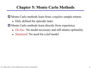
2. Monte Carlo Methods • Does not assume complete knowledge of the environment • Requires only “experience” – samples of states, actions and rewards – to be complete. • MC methods are ways of solving the RL problem based on averaging sample returns over episodic tasks. (For example: five runs of an algorithm could constitute an episode, then 20 episodes a gathering of sample data to average) • Important ideas carry over from Dynamic Programming. The same value functions are computed (Vπ and Qπ), and these functions interact in similar ways to obtain optimality. • Steps are: policy evaluation, compute V and Q for a fixed π, policy improvement, and finally generalized policy iteration.

3. Policy Evaluation • Recall value of a state is that state’s expected cumulative future discounted reward when starting from that state. To estimate from experience, average the returns observed upon each visit to said state. • Every-visit and first-visit MC converge to V as the number of visits (or first visits) to s goes to infinity. • First-visit montecarlo method: average of the returns following first visits to a state s over an episode(the first time a state is visited during a single run) • Basic Monte Carlo Algorithm • Init: π = policy to be evaluated, V = an arbitrary state-value function • Returns(s), an empty list for all s in S. • Repeat forever: • Generate and episode using π • For each state s appearing in the episode: R = return following the first occurrence of s Append R to Returns(s) V(s) = avg(Returns(s))

4. Algorithm Example • Using the rudimentary gridworld shown below. Begin starting in the bottom left corner with a policy that (for the sake of this example) manages to successfully take the following actions from the corner (1,1). {right, right, up, up , right} • At each state the arbitrary value function returns the number shown in the box. • The loop runs and an episode is generated. For example, in the first episode say the path is followed successfully, none of the chances for other directions take effect. In the first move R is set to .2 and the list Returns(2,1) appends R. And the value at state (2,1) is the average, currently .2. • The loop runs continuously each time the value function will have changed slightly and after the first run through the numbers in the box will have altered. • Since the value function is arbitrary to begin with, as the averages refine it over time, the numbers in the boxes (representing returns) will alter and as the loop approaches infinity the Value function will converge to the best function for this gridworld. • Say over a period of a single episode the box (2,1) returns .2, .3, .2, and .4. This means that at the end of that episode the new value function will average these to .275 and this will reflect in the next episode run over the gridworld.

5. Policy Eval. Example • Consider blackjack. This game can be naturally formulated as an episodic finite MDP. Each game is an episode rewards being +1, -1, and 0 for win, lose, and draw. All rewards during play are zero and there is no time discount. • There are a total of 200 states using three variables: player’s current sum, dealer’s showing card, and whether or not player holds an ace. • Assume the player’s policy is to hit until the sum is 20 or 21. • To find the state value for this policy by a Monte Carlo approach, simulate many games using the policy and average the returns following each state.

6. Estimates of the state-value functions are shown below. States with a usable ace are less because they’re more rare.

7. Monte Carlo Estimation of Action Values • If a model is not available, then it is particularly useful to estimate action values rather than state values. Here the primary goal is to estimate Q*. • Here the policy evaluation problem is to estimate Qπ(s,a). The complication being that since the policy is fixed then many stat-action pairs are never visited. • This can be solved by “exploring starts”, where the start point of any episode is a random state-action pair, so in an infinite time frame all pairs are visited infinitely.

8. Monte Carlo Control • Approximating optimal policies • Start with a general policy and approximate value function. Value is altered over time to more closely approximate the value function of the current policy, and policy is improved over time with respect to the changing value function. • Policy improvement is done by making the policy greedy with respect to the current value function. In this case we have an action-value function, and therefore no model is needed to construct the greedy policy. For any action-value function , the corresponding greedy policy is the one that, for each , deterministically chooses an action with maximal -value: π(s) = argmaxaQ(s,a) • Policy improvement then can be done by constructing each πk+1 as the greedy policy with respect to Qπk. This ensures that the overall process converges to the optimal policy and value function as each πk+1 is better than πk • Algorithm alters to reflect these changes, policy is arbitrary. Value function is now Q(s,a) and begins arbitrary. As the loop runs for each state-action pair Q is updated using the avg of returns(s,a) and for each state in the episode the policy at a state s is the best action (evaluated by the Q function) available at that state.