1. Monte Carlo Simulation Methods - ideal gas

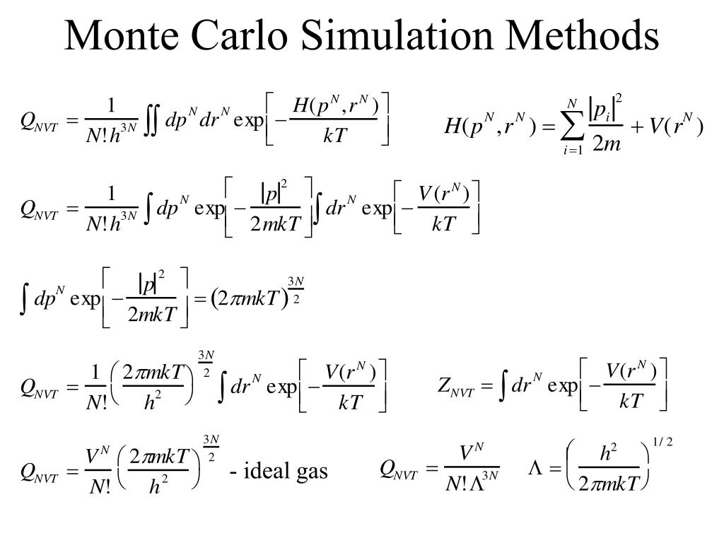
2. Calculating properties by integration

3. Theoretical background to Metropolis Markov chain of events: - the outcome of each trial depends only on the preceding trial - each trial belongs to a finite set of possible outcomes mn - probability of moving from state m to n =(1, 2,…. m, n,…N) - probability that the system is in a particular state (2)= (1).  (3)= (2). = (1). .  limit=limN (1) N - limiting (equilibrium) distribution mn - probability to choose the two states m,n between which the move is to be made (stochastic matrix). mn = mn. pmn - where p is the probability to accept the move mn = mn if n > m mn = mn. (n/m) if n < m and if n=m In practice if the energy of the n state is lower the move is accepted, if not a random number between 0 and 1 is compared to the Boltzmann factor exp(-∆V(rN)/kT). If the Boltzmann factor is greater then the Random number the move is accepted.

4. Implementation rand(0,1)≤ exp(-∆V(rN)/kT) Random number generators Linear congruential method