Monte Carlo Simulation

1. Monte Carlo Simulation Fawaz hrahsheh Dr. A. obeidat Department of physics just

2. History

3. What is Monte Carlo (MC) method ? • The Monte Carlo method :is a numerical method • for statistical simulation which utilizes sequences • of random numbers to perform the simulation

4. What the meaning of MC simulation? ●MC simulation is a versatile tool to analyse and evaluate complex measurements ● Constructing a model of a system. ●Experimenting with the model to draw inferences of the system’s behavior

5. A simulation model Measures of performance or behaviour of the system Decision and uncontrollable variables Simulation model outputs Inputs

6. A simulation model cont.. Model inputs capture the environment of the problem The simulation model Conceptual model: set of assumptions that define the system Computer code: the implementation of the conceptual model Outputs describe the aspects of system behaviour that we are interested in

7. Randomnumbers Uniform Random numbers or pseudo-random numbers (PRN) are essentially independent random variables uniformly Distributed over the unit interval (0,1). ●The PRNs are good if they are uniformly distributed, statistically independent and reproducible.

8. Linear congruential generator Generating a random sequence of numbers {X1,X2,…….,Xk} of length M over the interval [0,M-1] Xi=mod(AXi-1+C,M) R=Xi/M ♠♠♠ mod(b,M)=b-int(b/M)*M ● Starting value X0 is called “seed” ●M,A and C are nonnegative integers known Modulus, multiplier and increment, respectively ●M is must be prime number(2³¹-1,2-1,…..)

9. Fortran program program random_num implicit none integer,parameter::m=2**21,a=17,c=43 integer::i,n,s real(8)::R,Xo read*,n !n is the number of random points Xo=27.0d0 !------------------------ do i=1,n s=A*Xo+c Xo=mod(s,m) R=Xo/m write(*,*) R end do !------------------------ end program random_num

10. Classic Example Find the value of ? Use the reject and accept method Or hit and miss method The area of square=(2r)² The area of circle = r²

11. Cont.... Hit and miss algorithm ♣ Generate two sequences of N of PRN :: Ri,,Rj ♣ Xi=-1+2R i ♣ Yj=-1+2Rj ♣ Start from s=zero ♣ If (X²+Y²<1) s=s+1 ♣ # of dots inside circle=s ♣ total number of dots=N

12. Fortran program PROGRAM Pi implicit none integer,parameter::mm=(2**17)-1,aa=(2**7)-1 REAL(8)::X, Y, Pi Real(8),dimension(:),allocatable::R INTEGER::I,N Pi = 0.0d0 READ*, N allocate(R(n)) DO I = 1,N CALL RANDOM_NUMBER(R(n)) CALL RANDOM_NUMBER(R(n+1)) X =-1.0d0+2.0d0*R(n) Y=-1.0d0+2.0d0*R(N+1) IF (X*X+Y*Y<1.0d0) Pi=Pi+1.0d0 END DO Pi=4*Pi/N PRINT*,Pi END program pi

13. Monte Carlo Integration ♥ Hit and miss method ♥ Sample mean method ♥ importance sampled method

14. Hit and Miss method ♦Generate two sequence of N of PRN (Ri,R j) i& j=1,2,….,N ♦0 ≤f(x) ≤Ymax ,for X Є (a,b) ♦ Xi=a+Ri (b-a) ♦ Yi=Ymax R j ♦ start from s=0 ♦ if Yj<f(x) s=s+1 ♦I=Ymax(b-a) S/N

15. program Hit_miss implicit none real(8),dimension(:),allocatable::R real(8)::X,Y,m,a,b,integ integer::i,N,s read*,a !the lower value of the interval read*,b !the upper value of the interval M=f(b) if (dabs(f(a))>dabs(f(b))) M=f(a) read*,N !the number of random numbers allocate(R(n)) s=0 do i=1,N call random_number(R(n)) call random_number(R(n+1)) X=a+R(n)*(b-a) Y=M*R(n+1) if (y<f(x)) s=s+1 end do INTEG=M*(b-a)*s/N print*,integ contains real(8) function F(X) real(8),intent(in)::X F=2.0*X+1.0 end function F end program Hit_miss

16. Cont…. If there is a part of the function under X-axis This must now be corrected for the fact that the line y = -R has been used as the baseline for the integral instead of the line y = 0. This is accomplished by subtracting the rectangular area R(b-a). then

17. Types of distribution Uniform distribution Gaussian or normal distribution

18. Sample Mean method Rewrite By Where is p.d.f Theorem…. If x1,x2,x3,…..,xN are i,i,d uniformly distributed on [a,b],then ,

19. Cont… From the theorem choose and Then an estimate of I is You can calculate the value of error from the variance F(x) x a b

20. Sample Mean MC algorithm ♠ Generate sequence of N of PRN : Ri ♠Compute Xi=a+Ri (b-a) ♠ compute f(Xi) , i=1,2,3,….,N ♠ use ♠♠♠ note:: if f(x) is not square integrable ,then the MC Estimate Î will still converge to the true value, but The error estimate becomes unreliable.

21. program Sampled_Mean implicit none real(8),dimension(:),allocatable::R real(8)::a,b,sum,integ,X integer::i,N read*,a ! Lower value read*,b ! upper value read*,n ! number of random points allocate(R(n)) sum=0.0d0 do i=1,n call random_number(R(n)) call random_number(R(n+1)) X=a+R(n)*(b-a) sum=sum+f(x) int=((b-a)/N)*sum end do write(*,*) "integ=",integ contains real(8) function F(X) real(8),intent(in)::X F=2*X+1.0d0 end function F end program Sampled_Mean

22. Generalization to multidimensional cases Rewrite d-dimension integral by Because the uniform distribution ,choose and The estimate of I is

23. Importance Sampled method ●It is quite obvious that most of the integral comes from the region of the peak. But if we generate points evenly in the interval [a, b], most points won’t be in the peak area ,and their contribution to the total will be relatively small…. ●The idea behind importance sampling is to transform f(x) into another, flatter function which is then MC integrated of course there has to be a back-transformation to give the original integral we really want.

24. Important properties of continuous and discrete pdf ’s

25. Steps of Importance Sampled method by rewrite where where Now make a variable change and Then

26. Cont…. now the value of the integration equal to the average value The error calculated by variance method ♠♠♠ note that, the function must be invertible

27. Example (Importance-Sampled method ) find In this region, the function decreases from 1 to 1/e. The simple exponential function does the same, so let’s use that for g(x) . We first have to normalize g , so we calculate Then our normalized weighting function is

28. Cont.... let Then

29. Cont… ♣♣♣ note:: from the last result we redistribute the PRN according to the pdf (g(x)) , then the new values (i.e., ) are uniform random numbers used To find the value of on the interval of integration ,where the average value is the estimator value for the original integral.

30. program important_sample implicit none real(8)::sum,u,R,integ integer::i,N read*,N sum=0.0 do i=1,N call random_number(R) u=G_inv(R) sum=sum+f(u)/g(u) end do integ=sum/N write(*,*) integ contains real(8) function F(x) real(8),intent(in)::x F=dexp(-x**2) end function F real(8) function g(x) real(8),intent(in)::x g=dexp(-x) end function g real(8) function G_inv(x) real(8),intent(in)::x G_inv=-dlog(1-x*1.718d0/2.718d0) end function G_inv end program important_sample

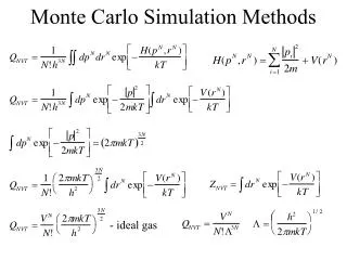
31. Why monte carlo ? MC is from the best methods to find the partition function numerically , then you can solve the stochastic processes.

32. Suppose we want to solve the following integral Using any other numerical method ,(i.e. Trapezoidal or Simpson) Where i=1,2,3,……,30 So we generate a grid in the domain of integration ,suppose a grid with 10 nodes on each coordinate axis in 30 dimension cube [ 0,1] ³º be chosen .in this case, we have 10³º abscissas. Suppose a time of 10 ־ second is necessary for calculating One value of the function . Therefore , a time of 10¹ years will be necessary for evaluating the integral.

33. Thank you