Understanding Random Variables: Indicator, Derived, and Continuous Transformations
This document elaborates on the concept of random variables (RVs) with a focus on Indicator RVs, Derived RVs, and Continuous RV Transformations. The discussion includes mean and variance calculations, the binomial distribution, and applications in fields such as genetics, particularly EST libraries. Key statistical principles like the Central Limit Theorem and order statistics are also examined, providing insights into how these concepts aid in probability analysis. Through practical examples, this guide aims to simplify complex statistical ideas for better understanding.

Understanding Random Variables: Indicator, Derived, and Continuous Transformations
E N D
Presentation Transcript
Probability: Many Random Variables (Part 2) Mike Wasikowski June 12, 2008
Contents • Indicator RV’s • Derived RV’s • Order RV’s • Continuous RV Transformations
Indicator RV’s • IA = 1 if event A occurs, 0 if not • Consider A1, A2, …, An events, I1, I2, …, In their indicator RV’s, and p1, p2, …, pn the probabilities of events Ai occurring • Then Σj Ijis the total number of events that occur • Mean of a sum of RV’s = sum of the mean of the RV’s (regardless of dependence), so E(Σj Ij) = Σj E(Ij) = Σj pj
Indicator RV’s • If all values of pi are equal, then E(Σj Ij) = np • When all events are independent, we calculate variance of number of events that occur as p1(1-p1)+…+pn(1-pn) • If all values of pi are equal and all events are independent, variance is np(1-p) • Thus, we have a binomial distribution
Ex: Sequencing EST Libraries • Transcription: DNA → mRNA → amino acids/proteions • EST (expressed sequence tag): a sequence of 100+ base pairs of mRNA • Different genes get expressed at different levels inside a cell • Abundance class L: where a cell contains L copies of an mRNA “species” • Generate an EST DB by sampling with replacement from the mRNA pool, see less rare species less often • How does the number of samples affect the proportion of rare species we will see?
Ex: Sequencing EST Libraries • Using indicator RV’s makes this problem easy to solve • Let Ia = 1 if a is in the S samples, 0 if not • Number of species in abundance class L = Σa Ia • We know each Ia has the same mean, so E(Σa Ia) = nLpL
Ex: Sequencing EST Libraries • Let pL = 1-rL, where rL is the probability this species is not in the database • rL = (1-L/N)S • Thus, we getE(Σa Ia) = nL(1- (1-L/N)S)
Derived RV’s • Previously saw how we find joint distributions and density functions • These joint pdf’s can be used to define many new RV’s • Sum • Average • Orderings • Because many statistical operations use these RV’s, knowing properties of their distributions is important
Sums and Averages • Two most important derived RV’s • Sn = X1+X2+…+Xn • X = Sn/n • Mean of Sn = nμ, variance = nσ2 • Mean of X = μ, variance = σ2/n • These properties generalize to well-behaved functions of RV’s and vectors of RV’s as well • Many important applicationsin probability and statisticsuse sums and averages
Central Limit Theorem • If X1, X2, ..., Xn are iid with a finite mean and variance, as n→∞, the standardized RV (X-μ)sqrt(n)/σ converges to an RV ~ N(0,1) Image from Wikipedia: Central Limit Theorem
Order Statistics • Involve the ordering of n iid RV’s • Call smallest X(1), next smallest X(2), up to biggest X(n) • Xmin =X(1), Xmax =X(n) • We know that these order statistics are distinct because P(X(i) = X(j)) = 0 for independent continuous RV’s
Minimum RV (Xmin) • Let X1, X2, ..., Xn be iid as X • If Xmin≥ x, then for each Xi, Xi≥ x • P(Xmin≥ x) = P(X ≥ x)n, also written as 1-Fmin(x) = (1-FX(x)) • By differentiating, we get the density function • fmin(x) = n fX(x)(1-FX(x))n-1
Maximum RV (Xmax) • Let X1, X2, ..., Xn be iid as X • If Xmax≤ x, then for each Xi, Xi≤ x • P(Xmax≤ x) = P(X ≤ x)n, also written as Fmax(x) = (FX(x))n • By differentiating, we get the density function • fmin(x) = n fX(x)(FX(x))n-1
Density function of X(i) • Let h be a small value, ignore events of probability o(h) • Consider the event that u < X(i) < u+h • In this event, i-1 RV's are less than u, one is between u and u+h, the remaining exceed u+h • Multinomial event with n trials and 3 outcomes • We have an approximation of P(u < X < u+h) ~ fX(u)h
Continuous RV Transformations • Consider n continuous RV's, X1, X2, ..., Xn • let V1 = V1(X1, X2, ..., Xn),V2, ..., Vn defined similarly • we then have a mapping from (X1, X2, ..., Xn) to (V1, V2, ..., Vn) • If the mapping is 1-1 and differentiable with a differentiable inverse, we can define the Jacobian matrix • Jacobian transformations are used to find marginal functions of one RV when that would be otherwise difficult • Used in ANOVA as well as BLAST