Download
1 / 41
410 likes | 562 Vues
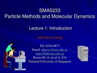
SMA5233 Particle Methods and Molecular Dynamics Lecture 1: Introduction A/P Chen Yu Zong Tel: 6516-6877 Email: phacyz@nus.edu.sg http://bidd.nus.edu.sg Room 08-14, level 8, S16 National University of Singapore. What is expected: .

E N D
SMA5233 Particle Methods and Molecular DynamicsLecture 1:Introduction A/P Chen Yu ZongTel: 6516-6877Email: phacyz@nus.edu.sghttp://bidd.nus.edu.sgRoom 08-14, level 8, S16 National University of Singapore
What is expected: • To learn basic theory, algorithm of molecular simulations and their applications • To learn the fundamentals in molecular modeling • To practice the installation and use of related software
Labs, Exams and Textbook: Projects and labs of part 1: • Molecular dynamics software (12%). • Simulation of biomolecular motions and dynamics (12%). Exams (part 1: 26%) Text and web: http://bidd.nus.edu.sg/group/teach/sma5233/sma5233.htm
Topics covered in part 1: • Lecture 1: Introduction • Lecture 2: Physical Principles and Design Issues of MD • Lecture 3: Force Fields • Lecture 4: Integration Methods • Lecture 5: Applications in Biomolecular Simulation and Drug Design
Topics covered in part 2: • Lecture 6, introduction to Monte Carlo method, random number generators • Lecture 7, Some applications of MC method • Lecture 8, Advanced MC methods, such as parallel tempering • Lecture 9, Brownian dynamics, stochastic differential equations • Lecture 10, dissipative particle method • Lecture 11, smoothed particle hydrodynamics
Reference Books for Part 1: • "Molcular Modelling. Principles and Applications". Andrew Leach. Publisher: Prentice Hall. ISBN: 0582382106. This book has rapidly become the defacto introductory text for all aspects of simulation. • "Molecular Dynamics Simulation: Elementary Methods". J.M. Haile. Publisher: Wiley. ISBN: 047118439X. This text provides a more focus but slightly more old-fashioned view of simulation. It has some nice simple examples of how to code (in fortran) some of the algorithms • P.W. Atkins Physical Chemistry (any edition) Chapters 11-14) • Schlick, T. Molecular Modeling and Simulation: An Interdisciplinary Guide. Springer-Verlag, New York, NY: 2002. ISBN 0-387-95404-X. • MacKerell, A.D., Jr., Empirical Force Fields for Biological Macromolecules: Overview and Issues, Journal of Computational Chemistry, 25: 1584-1604, 2004 • M. P. Allen, D. J. Tildesley (1989) Computer simulation of liquids. Oxford University Press. ISBN 0198556454. • J. A. McCammon, S. C. Harvey (1987) Dynamics of Proteins and Nucleic Acids. Cambridge University Press. ISBN 0-52-135652-0 (paperback); ISBN 0-52-130750 (hardback). • D. C. Rapaport (1996) The Art of Molecular Dynamics Simulation. ISBN 0521445612. • Daan Frenkel, Berend Smit (2001) Understanding Molecular Simulation. Academic Press. ISBN 0122673514. • J. M. Haile (2001) Molecular Dynamics Simulation: Elementary Methods. ISBN 047118439X • Oren M. Becker, Alexander D. Mackerell Jr, Benoît Roux, Masakatsu Watanabe (2001) Computational Biochemistry and Biophysics. Marcel Dekker. ISBN 082470455X. • Tamar Schlick (2002) Molecular Modeling and Simulation. Springer. ISBN 038795404X.
Molecular Modeling: Goals, Problems, Perspectives 1. Goal simulate/predict processes such as • DNA migration in nanofluidic tube • polypeptide folding thermodynamic • biomolecular association equilibria governed • partitioning between solvents by weak (nonbonded) • membrane/micelle formation forces • drug conformation
Example of MD Application:How can an enzyme metabolite escape? The enzyme acetylcholinesterase generates a strong electrostatic field that can attract the cationic substrate acetylcholine to the active site. However, the long and narrow active site gorge seems inconsistent with the enzyme's high catalytic rate. E + S E + P How does the metabolite P escape? Acetylcholinesterase (AChE) is the enzyme responsible for the termination of signaling in cholinergic synapses (such as the neuromuscular junction) by degrading the neurotransmitter acetylcholine. AChE has a gorge, 2 nm deep, leading to the catalytic site
How can an enzyme metabolite escape? Metabolite unlikely escape from the entrance How can it escape?
How can an enzyme metabolite escape? • How can it escape? • Can you tell which of the following possibilities is likely or unlikely, and why? • Protein unfolding • Condensation of ions on protein surface to counter-balance the force • Change of electric charge on metabolite • Alternative escape route
How can an enzyme metabolite escape? Alternative route An “open back door” policy: Transient opening of a channel to allow the metabolite to escape
MD simulation of acetylcholinesterase MD simulation clearly reveals transient opening of a channel “back door” Science 263, 1276-1278 (1994) The open “back door”allows the metabolite Pto escape
Molecular Modeling: Goals, Problems, Perspectives 1. Goal Common characteristics: • Degrees of freedom: atomic, coarse-grain (solute + solvent) Hamiltonian or • Equations of motion: classical dynamics force field • Governing theory:statistical mechanics entropy
Processes: Thermodynamic Equilibrium Folding Micelle Formation folded/native denatured micelle mixture Complexation Partitioning in membrane bound unbound in water in mixtures
Definition of a model for molecular simulation Every molecule consists of atoms that are very strongly bound to each other Degrees of freedom: atoms are the elementary particles Forces or interactions between atoms Boundary conditions MOLECULAR MODEL system temperature pressure Force Field =physicochemicalknowledge Methods for generating configurations of atoms: Newton
Molecular Modeling: Goals, Problems, Perspectives • Ensemble problem • Experimental problem A averaging B insufficient accuracy Four Problems • Force field A very small (free) energy differences B entropic effects C size problem • Search problem Athe search problem alleviated Bthe search problem aggravated
Four Problems • The Force Field Problem A very small (free) energy differences (kBT = 2.5 kJ/mol) resulting from summation over very many contributions (atoms) i i 106 – 108 must be very accurate B accounting for entropic effects not only energy minima are of importance but whole range of x-valueswith energies ~kBT must be included in the force field parameter calibration energy E(x) may have higher energy but lower free energy than coordinate x
Four Problems C size problem • The larger the system, the more accurate the individual energy contributions (from atoms) must be to reach the same overall accuracy • Calibrate force field using thermodynamic data for small molecules in the condensed phase keep force field physical + simple transferable computable
Choice of Model, Force Field, Sampling 3. Scoring Function, Energy Function, Force Field • Continuous n Lattice • Basis for force field or scoring function: 1. Structural data -Large molecules: crystal structures solution structures of proteins 2. Thermodynamic data -Small molecules: heat of vaporization, density in condensed phase partition coefficients e, D, h, etc. 3. Theoretical data - Small molecules: electrostatic potential and gradient in gas phase torsion–angle rotation profiles
Determination of Force Field Parameters Calibration sets of small molecules 1. Non-polar molecules 2. Polar molecules 3. Ionic molecules 2. Polar Molecules ethers, alcohols, esters, ketones, acids, amines, amides, aromatics, sulfides, thiols Calibration set: 28 compounds methanol ethanol 2-propanol butanol diethylether
ethylamine 1-butylamine ethyldiamine diethylamine n-methylacetamide acetone 2-butanone 3-pentanone acetic acid Determination of Force Field Parameters Calibration set: 28 compounds
Applications of Molecular Simulation in (Bio)Chemistry and Physics 2. Types of Processes • melting • adsorption • segregation • complex formation • protein folding • order-disorder transitions • crystallisation • reactions • protein stabilisation • membrane permeation • membrane formation • … 3. Types of Properties • structural • mechanical • dynamical • thermodynamical • electric • … • Types of Systems • liquids • solutions • electrolytes • polymers • proteins • DNA, RNA • sugars • other polymers • membranes • crystals • glasses • zeolites • metals • …
Objectives • Characterization of the populated microscopic states of molecules by molecular dynamics of spontaneous reversible motions in solution • Investigate the effect of • Thermodynamic conditions • Solvent environment • Amino acid composition, chain length on the peptide folding behavior • Characterization of the unfolded state
Four Problems 4.The Experimental Problem A Any experiment involves averaging over time and space (molecules) So it determines the average of a distribution, not the distribution itself However: Very different distributions may yield same average Example: circular dichroism(CD)-spectra b-peptides NOE’s + J-values of peptides in crystal solution • NOE: Nuclear Overhauser effect leads to changes in the intensity of signal(s) of a set of nuclei as a function of their respective distances. The use of NOE allows to obtain structural information on peptides and proteins in solution as well as the study of interactions between small ligands and biomolecules. probability P(Q) (linear) average <Q> quantity Q
Four Problems NOE’s: are notoriously insensitiveto the (atom-atom-distance) distribution provided a small part satisfies the NOE bounds J-values: may be sensitive to dihedral angle distribution X-ray: crystalcontains a much narrower distribution than a (aqueous) solution Experimental data cannot define a conformational ensemble B Experimental data have insufficient accuracy for force field calibration and testing accuracy of NOE’s, J-values, structure factors, etc. is limited but may improve with methodological and technical progress Example: NMR data on beta-hexapeptide, alpha-octapeptide Experimental data may converge over time towards simulation results
Molecular Simulations • Molecular Mechanics: energy minimization • Molecular Dynamics: simulation of motions • Monte Carlo methods: sampling techniques
What is molecular mechanics? • The term molecular mechanics refers to the use of Newtonian mechanics to model molecular systems. • Molecular mechanics approaches are widely applied in molecular structure refinement, molecular dynamics simulations, Monte Carlo simulations and ligand docking simulations. • Molecular mechanics can be used to study small molecules as well as large biological systems or material assemblies with many thousands to millions of atoms.
What is molecular mechanics? • All-atomistic molecular mechanics methods have the following properties: • Each atom is simulated as a single hard spherical particle • Each such particle is assigned a radius (typically the van der Waals radius) and a constant net charge (generally derived from high-level quantum calculations and/or experiment) • Bonded interactions are treated as "springs" with an equilibrium distance equal to the experimental or calculated bond length
What is molecular mechanics? • Molecular Mechanics (MM) finds the geometry that corresponds to a minimum energy for the system - a process known as energy minimization. • A molecular system will generally exhibit numerous minima, each corresponding to a feasible conformation. Each minimum will have a characteristic energy, which can be computed. The lowest energy, or global minimum, will correspond to the most likely conformation.
What is molecular dynamics simulation? • Simulation that shows how the atoms in the system move with time • Typically on the nanosecond timescale • Atoms are treated like hard balls, and their motions are described by Newton’s laws.
What is molecular dynamics simulation? • Beginning in theoretical physics, the method of MD gained popularity in material science and since the 1970s also in biochemistry and biophysics. • In chemistry, MD serves as an important tool in protein structure determination and refinement (see also crystallography, NMR) • In physics, MD is used to examine the dynamics of atomic-level phenomena that cannot be observed directly, such as thin film growth. It is also used to examine the physical properties of nanotechnology devices that have not or cannot yet be created.
What is molecular dynamics simulation? • Note that there is a large difference between the focus and methods used by chemists and physicists, and this is reflected in differences in the jargon used by the different fields. • In Chemistry, the interaction between the objects is either described by a force field (chemistry) (classical MD), a quantum chemical model, or a mix between the two. These terms are not used in Physics, where the interactions are usually described by the name of the theory or approximation being used.
Why MD simulations? • Link physics, chemistry and biology • Model phenomena that cannot be observed experimentally • Understand protein folding… • Access to thermodynamics quantities (free energies, binding energies,…)
Molecular Dynamics Simulations Schrödinger equation Born-Oppenheimer approximation Nucleic motion described classically Empirical force field
Molecular Dynamics Simulations Interatomic interactions
= = R Molecular dynamics Simulations of Biopolymers • Motions of nuclei are described classically, • Potential function Eel describes the electronic influence on motions of the nuclei and is approximated empirically „classical MD“: Covalent bonds Non-bonded interactions Eibond approximated exact KBT { 0 |R|
Computational task: Solve the Newtonian equations of motion:
Molecular dynamics is very expensive ... • Example: F1-ATPase in water (183 674 atoms), 1 nanosecond: • 106 integration steps • 8.4 * 1011 flop per step [n(n-1)/2 interactions] • total: 8.4 * 1017 flop • on a 100 MFLOPS workstation: 250 years • ...but performance has been improved by use of: • multiple time stepping 25 years • + structure adapted multipole methods 6 years • + FAMUSAMM 2 years • + parallel computers 55 days • FLOPS : Floating Point Operations Per Second on a standard benchmark such asLINPACK benchmark • Many other factors affect computation speed: I/O, inter-processor communication, cache coherence, memory hierarchy. • Typical systems: 2GHz Pentium 4 (few GFLOPS); IBM Blue Gene/L 131,072 processors (207.3 TFLOPS); SETI@home (100 TFLOPS); Pocket calculator (10 FLOPS); Human (milliFLOPS)
Limits of MD-Simulations • Classical description: Chemical reactions not described Poor description of H-atoms (proton-transfer) Poor description of low-T (quantum) effects Simplified electrostatic model Simplified force field • Only small systems accessible (104 ... 106 atoms) • Only short time spans accessible (ps ... μs)
MD as a tool for minimization Energy Molecular dynamics uses thermal energy to explore the energy surface State A State B position Energy minimization stops at local minima
Crossing energy barriers State B I Energy Position DG State A A B time Position The actual transition time from A to B is very quick (a few pico seconds). What takes time is waiting. The average waiting time for going from A to B can be expressed as: