Multicollinearity

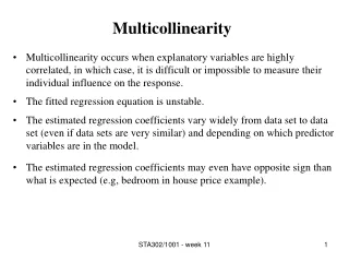
1. Multicollinearity • Multicollinearity - violation of the assumption that no independent variable is a perfect linear function of one or more other independent variables. • β1 is the impact X1 has on Y holding all other factors constant. If X1 is related to X2 then β1 will also capture the impact of changes in X2. • In other words, interpretation of the parameters becomes difficult.

2. Perfect vs. Imperfect • With perfect multicollinearity one cannot technically estimate the parameters. • Dominant variable - a variable that is so highly correlated with the dependent variable that it completely masks the effects of all other independent variables in the equation. • Example: Wins = f(PTS, DPTS) • Any other explanatory variable will tend to be insignificant. • Imperfect Multicollinearity - a statistical relationship exists between two or more independent variables that significantly affects the estimation of the model.

3. Consequences of Multicollinearity • Estimates will remain unbiased: • Estimates will still be centered around the true values. • The variances of the estimates will increase. • In essence we are asking the model to tell us something we know very little about (i.e. what is the impact of changing X1 on Y holding everything else constant). • Because we are not holding all else constant, the error associated with our estimate increases. • Hence it is possible for us to observe coefficients of the opposite sign than expected due to multicollinearity. • The computed t-stat will fall • Variance and standard error are increased. WHY?

4. More Consequences • Estimates will become very sensitive to changes in specification • Overall fit of the equation will be generally unaffected. • If the multicollinearity occurs in the population as well as the sample, then the predictive power of the model is unaffected. • Note: It is possible that multicollinearity is a result of the sample, so the above may not always be true. • The severity of the multicollinearity worsens its consequences.

5. Detection of Multicollinearity • High R2 with all low t-scores • If this is the case, you have multicollinearity. • If this is not the case, you may or may not have multicollinearity. • If all the t-scores are significant and in the expected direction than we can conclude that multicollinearity is not likely to be a problem. • High Simple Correlation Coefficients • A high r between two variables (.80 is the rule of thumb) indicates the potential for multicollinearity. In a model with more than two independent variables, though, this test will not tell us if a relationship exists between a collection of independent variables.

6. Variance Inflation Factor • Run an OLS regression that has Xi as a function of all the other explanatory variables in the equation. • Calculate the VIF VIF(βi) = 1 / (1-R2) • Analyze the degree of multicollinearity by evaluating the size of VIF. • There is no table of critical VIF values. The rule of thumb is if VIF > 5 then multicollinearity is an issue. Other authors suggest a rule of thumb of VIF > 10. • What is the R2 necessary to reach the rules of thumb?

7. Remedies • Do nothing • If you are only interested in prediction, multicollinearity is not an issue. • t-stats may be deflated, but still significant, hence multicollinearity is not significant. • The cure is often worse than the disease. • Drop one or more of the multicollinear variables. • This solution can introduce specification bias. WHY? • In an effort to avoid specification bias a researcher can introduce multicollinearity, hence it would be appropriate to drop a variable.

8. More Remedies • Transform the multicollinear variables. • Form a linear combination of the multicollinear variables. • Transform the equation into first differences or logs. • Increase the sample size. • The issue of micronumerosity. • Micronumerosity is the problem of (n) not exceeding (k). The symptoms are similar to the issue of multicollinearity (lack of variation in the independent variables). • A solution to each problem is to increase the sample size. This will solve the problem of micronumerosity but not necessarily the problem of multicollinearity.

9. Heteroskedasticity • Heteroskedasticity - violation of the classic assumption that the observations of the error term are drawn from distributions that have a constant variance.

10. Why does this occur? • Substantial differences in the dependent variables across units of observation in the cross-sectional data set. • People learn over time. • Improvements in data collection over time • The presence of outliers (an observation that is significantly different than all other observations in the sample).

11. Pure Heteroskedasticiy • Classic assumption: Homeoskedasticity or • var(ei) = σ2 = a constant • If this assumption is violated then var(ei) = σi2 • What is the difference? The variance is not a constant but varies across the sample. • The precise form of heteroskedasticity can take on a variety of forms. Our discussion will focus primarily on one form. • Proportionality factor (Z) - variance of the error term changes proportionally to some factor (Z). • Therefore var(ei) = σ2Zi

12. Consequences • Pure heteroskedasticity does not cause bias in the coefficient estimates • The variance of the coefficient estimates is now a function of the proportionality factor. Hence the variance of the estimates of β increases. These estimates are still unbiased, since over-estimation and under-estimation are still as likely. • Heteroskedasticity causes OLS to underestimate the variances (and standard errors) of the coefficients. • This is true as long as increases in the independent variable is related to increases in the variance of the error term. This positive relationship will cause the standard error of the coefficient to be biased negatively. In most economic applications, this is the nature of the heteroskedasticity problem. • Hence the t-stats and F-stats can not be relied upon for statistical inference.

13. Testing for Heteroskedasticity:First Questions • Are there any specification errors? • Is research in this area prone to the problem of heteroskedasticity? Cross-sectional studies tend to have this problem. • Does a graph of the residuals show evidence of heteroskedasticity?

14. Park Test • Estimate the model and save the residuals. • Log the squared residuals and regress these upon the log of the proportionality factor (Z). • Use the t-test to test the significance of Z. • PROBLEM: Picking Z

15. White Test • Estimate the model and save the residuals. • Square the residuals (don’t log) and regress these on each X, the square of each X, and product of each X times every other X. • Use the chi-square test to test the overall significance of the equation. The test stat is NR2, where N is the sample size and R2 is the unadjusted R2. Degrees of freedom equals the number of slope coefficients in equation. • If the test stat is larger than the critical value, reject the null hypothesis and conclude that you probably have heteroskedasticity. • I GOT MORE TESTS!!!

16. Remedies for Heteroskedasticity • Use weighted least squares. • Dividing the dependent and independent variables by Z will remove the problem of heteroskedasticity. • This is a form of generalized least squares. • Problem: How do we identify Z? • How do we identify the form of Z? • White’s heteroskedasticity-consistent variances and standard errors • The math is beyond the scope of the class, but statitical packages (like E-Views) do allow you to estimate the standard errors so that asymptotically valid statistical inferences can be made about the true parameter values.

17. More Remedies • Estimate a linear model with a double-logged model. • Such a model may be theoretically appealing since one is estimating the elasticities. • Logging the variables compresses the scales in which the variables are measured hence reducing the problem of heteroskedasticity. • In the end, you may be unable to resolve the problem of heteroskedasticity. In this case, report White’s heteroskedasticity-consistent variances and standard errors and note the substantial efforts you made to reach this conclusion

18. Serial Correlation • Which classic assumption are we talking about? • The correlation between any two observations of the error term is zero. • Issue: Is et related to et-1? Such would be the case in a time-series when a random shock has an impact over a number of time periods. • Why is this important? Y = a + bX + et • With serial correlation, et = f(et-1) • hence Y = f(Xt, et, et-1) • Therefore, serial correlation also impacts the accuracy of our estimates of the parameters.

19. Pure Serial Correlation • Pure serial correlation - a violation of the classical assumption that assumes uncorrelated observations of the error term. • In other words, we assume cov(ei, ej) = 0 • If the covariance of two error terms is not equal to zero, then serial correlation exists.

20. First Order Serial Correlation • The most common form of serial correlation is first order serial correlation. • et = ρet-1 + ut • where e = error term of the equation in question • ρ = (rho) parameter depicting the functional relationship between observations of the error term. • u = classical (non-serially correlated) error term

21. Strength of Serial Correlation • Magnitude of ρ indicates the strength of the serial correlation. • If ρ = 0 no serial correlation • as ρ approaches 1 in absolute value, the more the error terms are serially correlated. • If ρ > 1 then the error term continually increases over time, or explodes. Such a result is unreasonable. • So we expect -1 < ρ < 1 • Values greater than zero indicate positive serial correlation values less than zero indicate negative serial correlation. • Negative serial correlation indicates that the error term switches signs from observation to observation. • In the data utilized most commonly in economics, negative serial correlation is not expected.

22. Consequences • Pure serial correlation does not cause bias in the coefficient estimates • Serial correlation increases the variance of the β distributions • Pure serial correlation causes the dependent variable to fluctuate in a fashion that the estimation procedure (OLS) attributes to the independent variables. Hence the variance of the estimates of β increases. These estimates are still unbiased, since over-estimation and under-estimation are still as likely • Serial correlation causes OLS to underestimate the variances (and standard errors) of the coefficients. • Intuitively - Serial correlation increases the fit of the model. Hence the estimation of the variance and standard errors is lower. This can lead the researcher to conclude a relationship exists when in fact the variables in question are unrelated. • Hence the t-stats and F-stats can not be relied upon for statistical inference. • Spurious Regressions. REMEDIES???