Understanding Multicollinearity in Regression Analysis
This text discusses the nature, consequences, and solutions of multicollinearity in regression analysis, with examples and implications for OLS estimators. Learn how to detect, solve, and interpret imperfect multicollinearity in your data.


Understanding Multicollinearity in Regression Analysis
E N D
Presentation Transcript
The Nature of the Problem OLS requires that the explanatory variables are independent of error term • But they may not always be independent of each other. • Multicollinearity: data on explanatory variables for sample are perfectly or highly correlated • Perfect colinearity is when tow of the X variables are the same • STATA automatically controls for this by dropping one of them • Perfect Collinearity: Coefficients are indeterminate; SE are infinite • High degree of collinearity: large SE, imprecise coefficients, large interval estimation • Multiple Regression analysis: Cannot isolate independent effects i.e. hold one variable constant while changing the other. • OLS estimators still BLUE • Implications: • Large Variances and Covariances of estimators: • Large confidence intervals • Insignificant t-statistics • Non-rejection of zero-coefficient hypothesis • P(Type II error) large • F-Tests fail to reject joint insignificance • R2 high • Estimators and SE sensitive to few obs/data points • Detecting Multicollinearity • High R2/insignificant t-tests/significant F-Tests • High correlation coefficients between sample data on variables • Solve Multicollinearity: • Impose Economic Restrictions e.g CRS in CD production function • Improve Sample data • Drop variable (risk of mis-specifying model and having omitted variable bias) • Use rates of change of variables (impact on error term)
The Consequences • This is not a violation of the GM theorem • OLS is still BLUE and consistent • The standard errors and hypothesis tests are all still valid • So what is the problem? • Imprecision
Imprecision • Because the variables are correlated the move together • Therefore OLS cannot determine the partial effect with much reliability • Difficult to isolated specific effect of one variable when the tend to move together • This manifests itself as high standard errors • Equivalently the confidence intervals are very wide • Recall: CI=b+/-t*se
Perfect MC • Extreme example • Attempt a regression where one variable is perfectly correlated with another • Standard errors would be infinite because it would be impossible to separate the independent effects of the two variables which move exactly together • Stata will spot perfect multicolineararity and drop one variable • Can also happen if one variable is linear combination of others
Perfect Multicolinearity gen x2=inc_pc (1 missing value generated) . regress price inc_pchstock_pc x2 Source | SS df MS Number of obs = 41 -------------+------------------------------ F( 2, 38) = 210.52 Model | 6.7142e+11 2 3.3571e+11 Prob > F = 0.0000 Residual | 6.0598e+10 38 1.5947e+09 R-squared = 0.9172 -------------+------------------------------ Adj R-squared = 0.9129 Total | 7.3202e+11 40 1.8301e+10 Root MSE = 39934 ------------------------------------------------------------------------------ price | Coef. Std. Err. t P>|t| [95% Conf. Interval] -------------+---------------------------------------------------------------- inc_pc | 16.15503 2.713043 5.95 0.000 10.66276 21.6473 hstock_pc | 124653.9 389266.5 0.32 0.751 -663374.9 912682.6 x2 | (dropped) _cons | -190506.4 80474.78 -2.37 0.023 -353419.1 -27593.71 ------------------------------------------------------------------------------
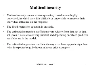
Imperfect Multicolinearity • If two (or more) x variables are highly correlated – but not perfectly correlated, stata wont drop them but the standard errors will be high • The implications • CI wider • more likely to not reject null hypothesis • Variables will appear individually statistically insignificant • But they will be jointly significant (F-test)
Detecting MC • Low t-statistics for individual tests of significance • High F-statistic for test of joint significance • High R2 • All these signs suggest that the variables matter collectively but it is difficult to distinguish their individual effects.
An Example regress lnQlnKlnL Source | SS df MS Number of obs = 33 -------------+------------------------------ F( 2, 30) = 33.12 Model | 3.11227468 2 1.55613734 Prob > F = 0.0000 Residual | 1.4093888 30 .046979627 R-squared = 0.6883 -------------+------------------------------ Adj R-squared = 0.6675 Total | 4.52166348 32 .141301984 Root MSE = .21675 ------------------------------------------------------------------------------ lnQ | Coef. Std. Err. t P>|t| [95% Conf. Interval] -------------+---------------------------------------------------------------- lnK | .4877311 .7038727 0.69 0.494 -.9497687 1.925231 lnL | .5589916 .8164384 0.68 0.499 -1.108398 2.226381 _cons | -.1286729 .5461324 -0.24 0.815 -1.244024 .9866783 ------------------------------------------------------------------------------
The Example • Production function example • K and L tend to increase over time together • Economically they have independent effects • But we cannot estimate their separate effects reliably with this data • individually insignificant • Nevertheless, K and L matter jointly for output • High R2 • High F statistic: can reject the null of joint insignificance
What to Do about it? • Maybe nothing • OLS is still BLUE • Individual estimates imprecise but model could still good at prediction • Add more data in the hope of getting more precise estimates • Making use of consistency • The distribution gets narrower as sample size rises • Drop variable • Risk omitted variable bias