Ordinary Differential Equation

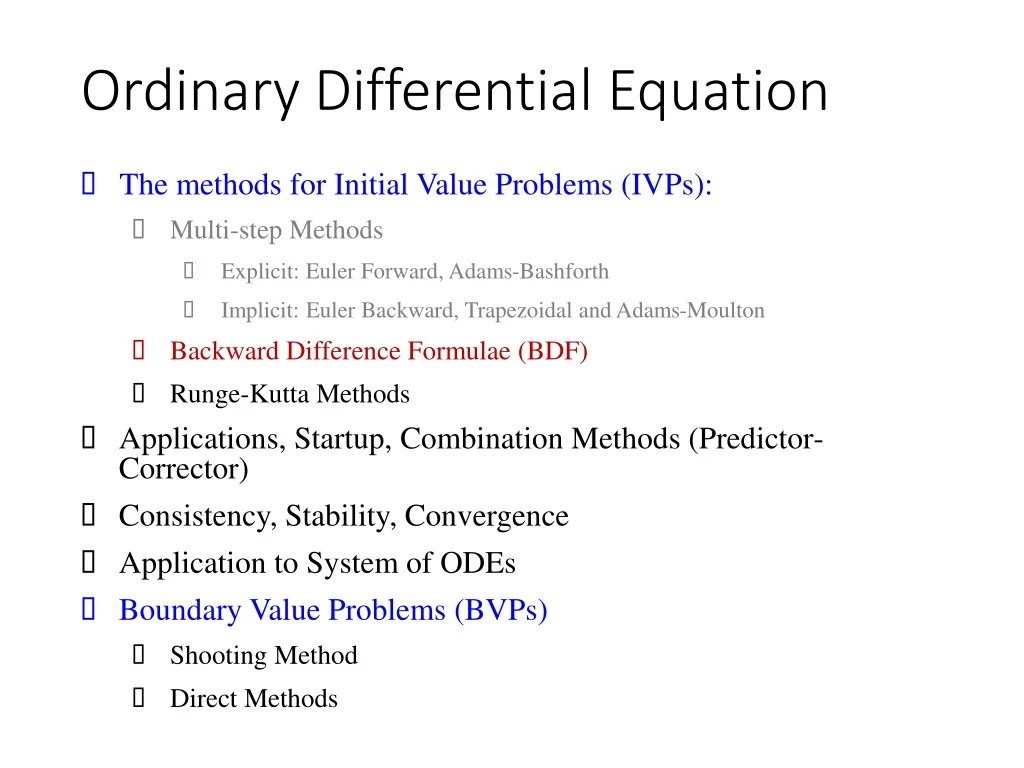
1. Ordinary Differential Equation • The methods for Initial Value Problems (IVPs): • Multi-step Methods • Explicit: Euler Forward, Adams-Bashforth • Implicit: Euler Backward, Trapezoidal and Adams-Moulton • Backward Difference Formulae (BDF) • Runge-Kutta Methods • Applications, Startup, Combination Methods (Predictor-Corrector) • Consistency, Stability, Convergence • Application to System of ODEs • Boundary Value Problems (BVPs) • Shooting Method • Direct Methods

2. ODE: Introduction We will consider general problems of the form: • Solution of this equation is a function y(t) • Starting from , we shall take discrete time steps of size h such that, • Starting from the known initial value , we shall compute values of y at each time step, , i.e., compute tab(y) • An obvious way can be: • Neglecting, h2 and higher order terms:

3. ODE: Introduction • The method is equivalent to making a forward difference approximation of dy/dt at the nth node. It is known as the Euler Forward Method. • Why not make a backward difference approximation of dy/dt at the nth node? This is known as the Euler Backward Method. • Instead of evaluating the function f either at the nth node or at the (n + 1)th node, if we take the average of the two:

4. ODE: Introduction • This method may also be seen as follows: • Left side integral is straight forward. Use Trapezoidal Method for the right side integral. This is known as the Trapezoidal Method.

5. , Multi-Step Methods: Explicit General form of multi-step or Adams-Bashforth methods: k = 0, 1, 2, …., n and h is the uniform time step size • Example: k = 3 Let’s expand all the terms in Taylor’s series and equate LHS with RHS!

6. , Multi-Step Methods: Explicit Thus, we have reduced to: Grouping Terms:

7. , Multi-Step Methods: Explicit Equating both sides:

8. , Multi-Step Methods: Explicit Thus, we have shown that effective approximation is: • Local truncation error (LTE) of this method is O(h4)! • The method is non-self starting, or cannot be started with the given initial condition y = y0 at t = t0 or 0. Why???

9. , Multi-Step Methods: Explicit Applying the first mean value theorem for integrals: Therefore, Global truncation error (GTE) of this method is O(h3)! A method is always referred to with it’s order of accuracy of GTE! Therefore, this is 3rd order Adams-Bashforth method!

10. , Multi-Step Methods: Explicit Some commonly used explicit methods:

11. , Multi-Step Methods: Implicit General form of multi-step implicit methods: k = 0, 1, 2, …., (n + 1) and h is the uniform time step size • Example: k = 2 Let’s expand all the terms in Taylor’s series and equate LHS with RHS!

12. , Multi-Step Methods: Implicit The method is: Using Taylor’s series expansion on both sides, we showed, The LTE of the method is O(h4) and GTE is O(h3). This is the 3rd order Adams-Moulton method!

13. , Multi-Step Methods: Implicit Some commonly used implicit methods:

14. , Backward Difference Formulae (BDF) So far, Explicit multi-step methods: k = 0, 1, 2, …., n and h is the uniform time step size And, Implicit multi-step methods: k = 0, 1, 2, …., (n + 1) and h is the uniform time step size All variations were in the evaluations of f. What happens if we keep the f evaluation at only one point and use multi-point approximation of the derivative dy/dt?

15. , Backward Difference Formulae (BDF) Backward Difference Formulae or BDFs: k = 0, 1, 2, …., (n + 1) and h is the uniform time step size • Example: k = 2 Let’s expand all the terms in Taylor’s series and equate LHS with RHS!

16. , Backward Difference Formulae (BDF) …(1) Differentiating (1),

17. , Backward Difference Formulae (BDF) Comparing LHS and RHS, the truncation error term is: The LTE of the method is O(h3) and the GTE is O(h2). This is the 2nd order BDF!

18. , Backward Difference Formulae (BDF)

19. Generalized Multi-Step Methods Mathematical Problem: All the multi-step (explicit and implicit) and BDF formulae derived so far can be expressed in a general form as follows: This will require a set of initial conditions Next, we shall derive a group of methods that deviate from this general framework!

20. , Runge-Kutta (R-K) Methods This is a group of Explicit methods that evaluates f at intermediate points within a time step h, i.e., between n and (n + 1). In generalized form, the method may be expressed as: where, ………

21. , Runge-Kutta (R-K) Methods Example: p = 1 Objective: estimate to achieve maximum accuracy, i.e., highest possible order of truncation error

22. , Runge-Kutta (R-K) Methods

23. , Runge-Kutta (R-K) Methods

24. , Runge-Kutta (R-K) Methods Therefore, one can derive infinitely many 2nd order R-K method. Most commonly used are the following three: • 2nd Order Runge-Kutta (aka Modified Euler, Midpoint method):

25. , Runge-Kutta (R-K) Methods • 2nd Order Runge-Kutta (aka Ralston’s method): • 2nd Order Runge-Kutta (aka Improved Euler, Heun’s method):

26. , Runge-Kutta (R-K) Methods Similarly, one can derive multiple 3rd and 4th order R-K methods. Two typically used algorithms for the 3rd and 4th order methods are as follow: • A 3rd Order Runge-Kutta Method:

27. , Runge-Kutta (R-K) Methods • A 4th Order Runge-Kutta Method: Let us now see applications of all the methods!

28. Runge-Kutta Methods for Numerical Integration Euler Method IV-order R-K Method Source: Surface Water-Quality Modeling, Chapra, Steven (1997).

29. Heun’s Method: Predictor-Corrector Source: Surface Water-Quality Modeling, Chapra, Steven (1997).

30. Ordinary Differential Equation • The methods for Initial Value Problems (IVPs): • Multi-step Methods • Explicit: Euler Forward, Adams-Bashforth • Implicit: Euler Backward, Trapezoidal and Adams-Moulton • Backward Difference Formulae (BDF) • Runge-Kutta Methods • Applications, Startup, Combination Methods (Predictor-Corrector) • Consistency, Stability, Convergence • Application to System of ODEs • Boundary Value Problems (BVPs) • Shooting Method • Direct Methods

31. , The Problem • Let us apply all the methods to the following IVP: • Analytical Solution

32. , Application: Multi-Step Methods (explicit) Some commonly used explicit methods:

33. , Euler Forward Continuing like this for 25 time steps to t = 10

34. , Adams-Bashforth (2nd Order) Continuing like this up to t = 10 From Euler Forward:

35. , Adams-Bashforth (3rd Order) Continuing like this up to t = 10

36. , Adams-Bashforth (4th Order) Continuing like this up to t = 10

37. , Euler Forward, Adams-Bashforth (2nd, 3rd and 4th Order)

38. Observations: explicit multi-step methods A few things to note for multi-step explicit methods: Euler Forward, Adams-Bashforth • All methods above the first order cannot start by themselves: • how to solve the start-up problem? • Some strange oscillation showing up in some of the methods (uncontrolled growth, instability): • Is there a system to this? • Can it be predicted? How to know when this will happen? • Can it be avoided? If yes, then how?

39. , Application: Multi-Step Methods (implicit) Some commonly used implicit methods:

40. , Euler Backward Continuing like this for 25 time steps to t = 10

41. , Trapezoidal Method Continuing like this up to t = 10

42. , Adams-Moulton (3rd Order)

43. , Adams-Moulton (4th Order)

44. , Euler Backward, Trapezoidal, Adams-Moulton (3rd and 4th Order)

45. Observations: implicit multi-step methods A few things to note for multi-step implicit methods: Euler Backward, Trapezoidal, Adams-Moulton • All methods above the second order cannot start by themselves. Accuracy of the higher order method is affected if the starting values are used from the lower order methods. • how to solve the start-up problem? • All implicit multi-step methods may involve solution of non-linear equations (if f contains a non-linear function of the dependent variable y) • Is there a way to avoid this solution of non-linear equations? • No numerical oscillations (instability) observed in any of the implicit methods: • Why the same order explicit multi-step methods show oscillation but implicit ones don’t? • Do they show oscillation under any conditions or are they oscillation-proof under all conditions?

46. , Application: Backward Difference Formulae (BDF) 1st Order BDF is Euler Backward. Let’s apply the rest.

47. , BDF (1st and 2nd Order) • 1st Order (Euler Backward) • 2nd Order

48. , BDF (3rd and 4th Order) • 3rd Order • 4th Order

49. , BDF (5th and 6th Order) • 5th Order • 6th Order

50. , BDF (1st to 6th Order)