ImageJ
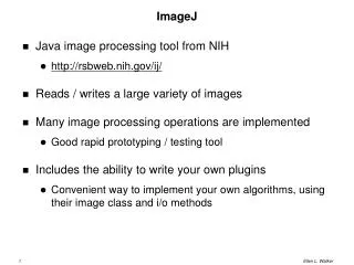
ImageJ. Java image processing tool from NIH http://rsbweb.nih.gov/ij/ Reads / writes a large variety of images Many image processing operations are implemented Good rapid prototyping / testing tool Includes the ability to write your own plugins

ImageJ
E N D
Presentation Transcript
ImageJ • Java image processing tool from NIH • http://rsbweb.nih.gov/ij/ • Reads / writes a large variety of images • Many image processing operations are implemented • Good rapid prototyping / testing tool • Includes the ability to write your own plugins • Convenient way to implement your own algorithms, using their image class and i/o methods
Point Processes • Pixel by pixel transformation • Output pixel depends only on corresponding input pixel • Examples: • Out(r,c) = In(r,c) * 1.25 • Out(r,c) = In(r,c) + 25 • Out(r,c) = (In(r,c))2
Linear Transformations • Out(r,c) = In(r,c) * gain + bias • Gain controls contrast • Bias controls brightness • Location dependent: • Out(r,c) = In(r,c) * gain(r,c) + bias(r,c) • E.g. “sky darkening filter” • Linear Blend • Out(r,c) = (lambda) * In1(r,c) + (1-lambda) * In2(r,c) • If In1 and In2 are images, a sequence of these from lambda = 0 to lambda=1 is an image dissolve
Histogram • An image histogram counts the number of pixels at each brightness. • Color images have 3 histograms (red, green, blue)
Information in Histogram • Contrast (variation in brightness) • Are bars spread over the whole range? • Foreground vs. background color • Are there two separate “peaks” with a valley between?
Applications of Histogram • Thresholding • Find a value that separates foreground / background values • Look for a “valley” between two peaks (may or may not be what you need) • Contrast enhancement • Histogram equalization – spread the data as evenly through the histogram as possible • Goal: wide, flat histogram
Example: Histogram Equalization • Original • Modified
Algorithm: Histogram Equalization • Find cumulative distribution • For each intensity I, c(I) = # pixels <= I • Code: C[0]=Hist[0]; For(greylevel =1; greylevel < max; greylevel++){ C[greylevel] = Hist[greylevel] + C[greylevel-1]; C[greylevel] = C[greylevel] / (double)(rows*cols); }
Algorithm: Histogram Equalization • Use C(I) as a lookup table to determine the final value of each pixel. • Since C(I) ranges from 0 to 1 (why?), multiply C(I) by the max pixel value to get the output value • Code: For(r=0;r<rows;r++) for(c=0;c<cols;c++) out[r][c] = C[(in[r][c])]*MAX;
Locally Adaptive Histogram Equalization • Instead of doing histogram equalization using the whole image, compute the distribution for a moving window around the given pixel. • Avoids effect of bright light at one corner washing out everything in the image.
N W E S Image Neighborhoods • Neighborhoods can be defined for each pixel • The two most common neighborhoods • 4-neighborhood • 8-neighborhood
Applying a Mask • Mask is a set of relative pixel positions. One is designated the origin (0,0) - usually at center • Each mask element is weighted • To apply the mask, put the origin pixel over the image pixel and multiply weights by the pixels under them, then add up all the values. • Usually this is repeated for every pixel in the image . Assumptions must be made for pixels near the edge of the image.
Mask application example • Result is 0 0 0 1 1 0 0 1 2 2 0 1 2 3 2 1 2 3 3 2 2 3 3 3 2 Boundary pixels are gray • Mask = 1 1 1 • Apply to every pixel in image: 0 0 0 0 1 0 0 0 1 1 0 0 1 1 1 0 1 1 1 1 1 1 1 1 1
Mathematical Representation of Mask Operations • Equation from Chapter 3 • g is the output image • f is the input image • h is the mask (also called kernel) • Short form (convolution operator)
Masks that "blur" • "Box mask" - every pixel gets the average of its neighborhood 1 1 1 After computing, divide by 9 (mask sum) 1 1 1 to keep image from getting too bright 1 1 1 • "Weighted average" - divide by 16 after application 1 2 1 2 4 2 1 2 1
Why blur? • Avoid effects of small random noise (“salt and pepper”) • Remove small features to emphasize larger ones • Bigger masks blur more / remove larger features • Sequence of masks generates sequence of increasingly blurred images (useful for some matching algorithms) • First step in sharpening the image (!) Sharp(x,y) = orig(x,y) + gamma (orig(x,y) – (blur * orig(x,y)))
Boundary Effects (padding) Figure 3.12
Common Masks Figure 3.13
Median Filtering • Example of a non-linear filter • Replace the central pixel of a window with the median pixel of the window • Compare to box filter, which replaces with average value in the window • Tends to preserve edges (why?)

