Topological Sort
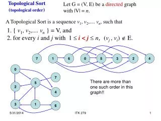
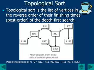
Topological sort is the list of vertices in the reverse order of their finishing times (post-order) of the depth-first search. Topological Sort. Possible topological sort: R37 R137 R51 R63 R53 R151 R173 R263.

Topological Sort
E N D
Presentation Transcript
Topological sort is the list of vertices in the reverse order of their finishing times (post-order) of the depth-first search. Topological Sort Possible topological sort: R37 R137 R51 R63 R53 R151 R173 R263
The topological sort uses the algorithm for dfs(), so its running time is also O(V+E), where V is the number of vertices in the graph and E is the number of edges. Running Time for Topological Sort
Any graph can be partitioned into a unique set of strong components. Strongly Connected Components
The algorithm for finding the strong components of a directed graph G uses the transpose of the graph. The transpose GT has the same set of vertices V as graph G but a new edge set consisting of the edges of G but with the opposite direction. Strongly Connected Components (continued)
Execute the depth-first search dfs() for the graph G which creates the list dfsList consisting of the vertices in G in the reverse order of their finishing times. Generate the transpose graph GT. Using the order of vertices in dfsList, make repeated calls to dfs() for vertices in GT. The list returned by each call is a strongly connected component of G. Strongly Connected Components (continued)
Strongly Connected Components (continued) dfsList: [A, B, C, E, D, G, F] Using the order of vertices in dfsList, make successive calls to dfs() for graph GT Vertex A: dfs(A) returns the list [A, C, B] of vertices reachable from A in GT. Vertex E: The next unvisited vertex in dfsList is E. Calling dfs(E)returns the list [E]. Vertex D: The next unvisited vertex in dfsList is D; dfs(D) returnsthe list [D, F, G] whose elements form the last strongly connected component..
strongComponents() // find the strong components of the graph; // each element of component is a LinkedList // of the elements in a strong component public static <T> void strongComponents(DiGraph<T> g, ArrayList<LinkedList<T>> component) { T currVertex = null; // list of vertices visited by dfs() for graph g LinkedList<T> dfsList = new LinkedList<T>(); // list of vertices visited by dfsVisit() // for g transpose LinkedList<T> dfsGTList = null; // used to scan dfsList Iterator<T> gIter; // transpose of the graph DiGraph<T> gt = null;
strongComponents()(continued) // clear the return vector component.clear(); // execute depth-first traversal of g dfs(g, dfsList); // compute gt gt = transpose(g); // initialize all vertices in gt to WHITE (unvisited) gt.colorWhite();
strongComponents()(continued) // call dfsVisit() for gt from vertices in dfsList gIter = dfsList.iterator(); while(gIter.hasNext()) { currVertex = gIter.next(); // call dfsVisit() only if vertex // has not been visited if (gt.getColor(currVertex) == VertexColor.WHITE) {
strongComponents()(concluded) // create a new LinkedList to hold // next strong component dfsGTList = new LinkedList<T>(); // do dfsVisit() in gt for starting // vertex currVertex dfsVisit(gt, currVertex, dfsGTList, false); // add strong component to the ArrayList component.add(dfsGTList); } } }
Recall that the depth-first search has running time O(V+E), and the computation for GT is also O(V+E). It follows that the running time for the algorithm to compute the strong components is O(V+E). Running Time of strongComponents()
Dijkstra's algorithm computes minimum path weight from a specified vertex toall other vertices in the graph. The breadth‑first search can be used to find the shortest path from a specific vertex to all the other vertices in the graph. Minimum spanning tree for a connected, undirected graph is the set of edges that connect all vertices in the graph with the smallest total weight. Graph Optimization Algorithms
The breadth-first search can be modified to find shortest paths. Begin at vertex sVertex and visit its neighbors (path length 1) followed by vertices with successively larger path lengths. The algorithm fans out from sVertex along paths of adjacent vertices until it visits all vertices reachable from sVertex. The Shortest Path Algorithm
Each vertex must maintain a record of its parent and its path length from sVertex. The DiGraph class provides methods that allow the programmer to associate two fields of information with a vertex. One field identifies the parent of a vertex and the other field is an integer dataValue associated with the vertex. The method initData() assigns a representation for to each dataValue field of the graph vertices. The Shortest Path Algorithm (continued)
A breadth‑first search visit to a vertex defines a path of shortest length from the starting vertex. The parent field of the vertex determines the order of vertices from the starting vertex. The Shortest Path Algorithm (continued)
The minimum path problem is to determine a path of minimum weight from a starting vertex vs to each reachable vertex in the graph. The path may contain more vertices than the shortest path from vs. Dijkstra's Minimum-Path Algorithm
Dijkstra's Minimum-Path Algorithm (continued) Three paths, A-B-E, A-C-E, and A-D-E, have path length 2, with weights 15, 17, and 13 respectively. The minimum path is A-C-D-E, with weight 11but path length 3.
Define the distance from every node to the starting node: Initially the distance is 0 to the starting node and infinity to other nodes. Use a priority queue to store all the nodes with distance (the minimal distance node on the top). Each step in the algorithm removes a node from the priority queue and update the distance to other nodes in the queue via this node. Dijkstra's Minimum-Path Algorithm (continued)
Since no subsequent step could find a new path to the node with a smaller weight (because the weights are positive), we have found the minimum path to this node. Repeat this above step and the algorithm terminates whenever the priority queue becomes empty. Dijkstra's Minimum-Path Algorithm (continued)
Dijkstra's algorithm has running time O(V + E log2V). Running Time of Dijkstra's Algorithm
When the weighted digraph is acyclic, the problem of finding minimum paths is greatly simplified. The depth-first search creates a list of vertices in topolocial order. dfsList : [v0, v1, . . .,vi, . . ., vn-1] Assume vi is the starting vertex for the minimum-path problem. Vertices in the list v0 to vi-1 are not reachable from vi. Minimum Path in AcyclicGraphs
After initializing the data value for all of the vertices to , set the data value for vi to 0 and its parent reference to vi. A scan of the vertices in dfsList will find that v0 through vi-1 have value and will not be considered. The algorithm discovers vi and iteratively scans the tail of dfsList, proceeding much like Dijkstra's algorithm. Minimum Path in AcyclicGraphs (continued)
At a vertex v in the sequential scan of dfsList, its current data value is the minimum path weight from vi to v. For there to be a better path, there must be an unvisited vertex, v', reachable from vi that has an edge to v. This is not possible, since topological order guarantees that v' will come earlier in dfsList. Minimum Path in AcyclicGraphs (continued)
The algorithm first creates a topological sort of the vertices with running time O(V+E). A loop visits all of the vertices in the graph once and examines edges that eminate from each vertex only once. Access to all of the vertices and edges has running time O(V+E) and so the total running time for the algorithm is O(V+E). Running Time for MinimumPath in Acyclic Graphs
A minimum spanning tree for a connected undirected graph is an acyclic set of edges that connect all the vertices of the graph with the smallest possible total weight. A network connects hubs in a system. The minimum spanning tree links all of the nodes in the system with the least amount of cable. Minimum Spanning Tree
The mechanics are very similar to the Dijkstra minimum-path algorithm. The iterative process begins with any starting vertex and maintains two variables minSpanTreeSize and minSpanTreeWeight, which have initial values 0. Each step adds a new vertex to the spanning tree. It has an edge of minimal weight that connects the vertex to those already in the minimal spanning tree. Prim's Algorithm
Prim's algorithm uses a priority queue where elements store a vertex and the weight of an edge that can connect it to the tree. When an object comes out of the priority queue, it defines a new edge that connects a vertex to the spanning tree. Prim's Algorithm (continued)
Like Dijkstra's algorithm, Prim's algorithm has running time O(V + E log2V). Running Time for Prim's Algorithm