Efficient FFTs On VIRAM
430 likes | 554 Vues
This presentation details the Fast Fourier Transform (FFT) and its significance in numerous applications like signal processing, multimedia, and scientific computing. It covers the implementations on the VIRAM architecture, comparing the "naïve" algorithm with three optimized versions. Performance results for both 32-bit floating-point and 16-bit fixed-point data are provided, demonstrating the capability of the VIRAM system. The discussion also explores the theory behind FFTs, DFT computation, and architectural assumptions, leading to conclusions and suggestions for future work.

Efficient FFTs On VIRAM
E N D
Presentation Transcript
Efficient FFTs On VIRAM Randi Thomas and Katherine Yelick Computer Science Division University of California, Berkeley IRAM Winter 2000 Retreat {randit, yelick} @cs.berkeley.edu
Outline • What is the FFT and Why Study it? • VIRAM Implementation Assumptions • About the FFT • The “Naïve” Algorithm • 3 Optimizations to the “Naïve” Algorithm • 32 bit Floating Point Performance Results • 16 bit Fixed Point Performance Results • Conclusions and Future Work
What is the FFT? The Fast Fourier Transform converts a time-domain function into a frequency spectrum
Why Study The FFT? • 1D Fast Fourier Transforms (FFTs) are: • Critical for many signal processing problems • Used widely for filtering in Multimedia Applications • Image Processing • Speech Recognition • Audio & video • Graphics • Important in many Scientific Applications • The building block for 2D/3D FFTs All of these are VIRAM target applications!
Outline • What is the FFT and Why Study it? • VIRAM Implementation Assumptions • About the FFT • The “Naïve” Algorithm • 3 Optimizations to the “Naïve” Algorithm • 32 bit Floating Point Performance Results • 16 bit Fixed Point Performance Results • Conclusions and Future Work
System on the chip: Scalar processor: 200 MHz “vanilla” MIPS core Embedded DRAM: 32MB, 16 Banks, no subbanks Memory Crossbar: 25.6 GB/s Vector processor: 200 MHz I/O: 4 x 100 MB/sec VIRAM Implementation Assumptions
LANE 3 LANE 1 LANE 4 LANE 2 64-bits 64-bits 64-bits 64-bits 32-bits 32-bits 32-bits 32-bits 32-bits 32-bits 32-bits 32-bits VL 5 VL 7 VL 2 VL 1 VL 6 VL 8 VL 3 VL 4 16 16 16 16 16 16 16 16 16 16 16 16 16 16 16 16 VL 15 VL 1 VL 13 VL 14 VL 10 VL 16 VL 2 VL 5 VL 6 VL 11 VL 7 VL 12 VL 3 VL 4 VL 9 VL 8 VIRAM Implementation Assumptions • VectorProcessor has four 64-bit pipelines=lanes • Each lane has: • 2 integer functional units • 1 floating point functional unit • All functional units have a 1 cycle multiply-add operation • Each lane can be subdivided into: • two 32-bit virtual lanes • four 16-bit virtual lanes
16-bit Integer 32-bit Integer 32-bit Single Precision All multiply-adds No multiply-adds All multiply-adds No multiply-adds All multiply-adds No multiply-adds Operations per Cycle 32 Integer 64 Integer 16 Integer 16 Floating Point 8 Floating Point 32 Integer 12.8 GOP/s 6.4 GOP/s 6.4 GOP/s 3.2 GOP/s 3.2 GFLOP/s 1.6 GFLOP/s Peak Performance Peak Performance • Peak Performance of This VIRAM Implementation • Implemented: • A 32 bit Floating point version (8 lanes, 8 FUs) • A 16 bit Fixed point version (16 lanes, 32 FUs)
Outline • What is the FFT and Why Study it? • VIRAM Implementation Assumptions • About the FFT • The “Naïve” Algorithm • 3 Optimizations to the “Naïve” Algorithm • 32 bit Floating Point Performance Results • 16 bit Fixed Point Performance Results • Conclusions and Future Work
Computing the DFT (Discrete FT) • Given the N-element vector x, its 1D DFT is another N-element vector y, given by formula: • where = the jkth root of unity • N is referred to as the number of points • The FFT (Fast FT) • Uses algebraic Identities to compute DFT in O(NlogN) steps • The computation is organized into log2N stages • for the radix 2 FFT
= X0 + w*XN/2 X0 . = X0 - w*XN/2 XN/2 . . . Computing A Complex FFT • Basic computation for a radix 2 FFT: • The basic computation on VIRAM for Floating Point data points: • 2 multiply-adds + 2 multiplies + 4 adds = • 8 operations • 2 GFLOP/s is the VIRAM Peak Performance for this mix of instructions • Xiare the data points • wis a “root of unity”
Vector Terminology • The Maximum Vector Length (MVL): • The maximum # of elements 1 vector register can hold • Set automatically by the architecture • Based on the data width the algorithm is using: • 64-bit data, MVL = 32 elements/vector register • 32-bit data, MVL = 64 elements/vector register • 16-bit data, MVL = 128 elements/vector register • The Vector Length (VL): • The total number of elements to be computed • Set by the algorithm: the inner for-loop
One More (FFT) Term! • Abutterfly group (BG): • A set of elements that can be computed upon in 1 FFT stage using: • The same basic computation AND • The same root of unity • The number of elements in a stage’s BG determines the Vector Length (VL) for that stage
Outline • What is the FFT and Why Study it? • VIRAM Implementation Assumptions • About the FFT • The “Naïve” Algorithm • 3 Optimizations to the “Naïve” Algorithm • 32 bit Floating Point Performance Results • 16 bit Fixed Point Performance Results • Conclusions and Future Work
Stage 3VL = 2 Stage 4VL = 1 Stage 2VL = 4 Stage 1VL = 8 vr1 vr1 vr2 vr1 vr2 vr1 vr2 vr2 Time Cooley-Tukey FFT Algorithm vr1+vr2=1butterfly group; VL = vector length
Diagram illustrates “naïve” vectorization A stage vectorizes well whenVL ³ MVL Poor HW utilization when VL is small(< MVL) Later stages of the FFT have shorter vector lengths: the # of elements in one butterfly group is smaller in the later stages Vectorizing the FFT Stage 3VL = 2 Stage 4VL = 1 Stage 2VL = 4 Stage 1VL = 8 vr1 vr1 vr2 vr1 vr2 vr1 vr2 vr2 Time
Naïve Algorithm: What Happens When Vector Lengths Get Short? • Performance peaks (1.4-1.8 GFLOPs) if vector lengths are ³ MVL • For all FFT sizes, 94% to 99% of the total time is spent doing the last 6 stages, when VL < MVL (= 64) • For 1024 point FFT, only 60% of the work is done in the last 6 stages • Performance significantly drops when vector lengths < # lanes (=8) 32 bit Floating Point VL=64=MVL
Outline • What is the FFT and Why Study it? • VIRAM Implementation Assumptions • About the FFT • The “Naïve” Algorithm • 3 Optimizations to the “Naïve” Algorithm • 32 bit Floating Point Performance Results • 16 bit Fixed Point Performance Results • Conclusions and Future Work
Optimization #1: Add auto-increment • Automatically adds an increment to the current address in order to obtain the next address • Auto-increment helps to: • Reduce the scalar code overhead • Useful: • To jump to the next butterfly group in an FFT stage • For processing a sub-image of a larger image in order to jump to the appropriate pixel in next row
Optimization #1: Add auto-increment • Small gain from auto-increment • For 1024 point FFT: • 202 MFLOP/s w/o AI • 225 MFLOP/s with AI • Still 94-99% of the time spent in last 6 stages where the VL < 64 • Conclusion: Auto-increment helps, but scalar overhead is not the main source of the inefficiency 32 bit Floating Point
256 3 128 5 > 2048 1 FFT Sizes 512 - 2048 2 Number of Transposes Needed Optimization #2: Memory Transposes • Reorganize the data layout in memory to maximize the vector length in later FFT stages • View the 1D vector as a 2D matrix • Reorganization is equivalent to a matrix transpose • Transposing the data in memory only works for N ³ (2 * MVL) • Transposing in memory adds significant overhead • Increased memory traffic • cost too high to make it worthwhile • Multiple transposes exacerbate the situation:
0 1 2 3 4 5 6 7 vr1 Stage 2: SWAP vr2 8 9 10 11 12 13 14 15 vr1 0 1 2 3 8 910 11 Stage 3: SWAP SWAP vr2 4 56 712 13 14 15 vr1 0 1 45 8 91213 Stage 4: SWAP SWAP vr2 2 36 71011 14 15 Optimization #3: Register Transposes • Rearrange the elements in the vector registers • Provides a way to swap elements between 2 registers • What we want to swap (after stage 1 VL = MVL = 8): VL = 4 BGs= 2 VL = 2 BGs= 4 • This behavior is hard to implement with one instruction in hardware
Optimization #3: Register Transposes • Two instructions were added to the VIRAM Instruction Set Architecture (ISA): • vhalfup andvhalfdn: both move elements one-way between vector registers • Vhalfup/dn: • Are extensions of already existing ISA support for fast in-register reductions • Required minimal additional hardware support • mostly control lines • Much simpler and less costly than a general element permutation instruction • Rejected in the early VIRAM design phase • An elegant, inexpensive, powerful solution to the short vector length problem of the later stages of the FFT
vr1 0 1 2 3 4 5 6 7 0 1 2 3 4 5 6 7 • move vr3 8 9 10 11 12 13 14 15 8 9 10 11 12 13 14 15 0 1 2 3 4 5 6 7 0 1 2 3 4 5 6 7 vr1 vr2 • vhalfup vr2 vr1 0 1 2 3 8 9 10 11 • vhalfdn vr3 vr2 4 5 6 7 12 13 14 15 Optimization #3: Register Transposes Stage 1: SWAP • Three steps to swap elements: • Copy vr1 into vr3 • Move vr2’s low to vr1’s high (vhalfup) • vr1 now done • Move vr3’s high to vr2’s low (vhalfdn) • vr2 now done
Optimization #3: Final Algorithm • The optimized algorithm has two phases: • Naïve algorithm is used for stages whose VL ³ MVL • Vhalfup/dn code is used on: • Stages whose VL < MVL = the last log2 (MVL) stages • Vhalfup/dn: • Eliminates short vector length problem • Allows all vector computations to have VL equal to MVL • Multiple butterfly groups done with 1 basic operation • Eliminates all loads/stores between these stages • Optimized vhalf algorithm does: • Auto-increment, software pipelining, code scheduling • the bit reversal rearrangements of the results • Single precision, floating point, complex, radix-2 FFTs
Optimization #3: Register Transposes • Every vector instruction operates with VL=MVL • For all stages • Keeps the vector pipeline fully utilized • Time spent in the last 6 stages • drops to 60% to 80% of the total time 32 bit Floating Point
Outline • What is the FFT and Why Study it? • VIRAM Implementation Assumptions • About the FFT • The “Naïve” Algorithm • 3 Optimizations to the “Naïve” Algorithm • 32 bit Floating Point Performance Results • 16 bit Fixed Point Performance Results • Conclusions and Future Work
Performance Results • Both Naïve versions utilize the auto-increment feature • 1 does bit reversal, the other does not • Vhalfup/dn with and without bit reversal are identical • Bit reversing the results slows naïve algorithm, but not vhalfup/dn 32 bit Floating Point
Performance Results • The performance gap testifies: • To the effectiveness of the vhalfup/dn algorithm in fully utilizing the vector unit • The importance of the new vhalfup/dn instructions 32 bit Floating Point
Performance Results • VIRAM is competitive with high-end specialized Floating Point DSPs • Could match or exceed the performance of these DSPs if the VIRAM architecture were implemented commercially 32 bit Floating Point
Outline • What is the FFT and Why Study it? • VIRAM Implementation Assumptions • About the FFT • The “Naïve” Algorithm • 3 Optimizations to the “Naïve” Algorithm • 32 bit Floating Point Performance Results • 16 bit Fixed Point Performance Results • Conclusions and Future Work
16 bit Fixed Point Implementation • Resources: • 16 lanes (each 16 bits wide) • Two Integer Functional Units per lane • 32 Operations/Cycle • MVL = 128 elements • Fixed Point Multiply-Add not utilized • 8 bit operands too small • 8 bits * 8 bits = 16 bit product • 32 bit product too big • 16 bits * 16 bits = 32 bit product
16 bit Fixed Point Implementation (2) • The basic computation takes: • 4 multiplies + 4 adds + 2 subtracts = 10 operations • 6.4 GOP/s is Peak Performance for this mix • To prevent overflow two bits are shifted right and lost for each stage Input Sbbb bbbb bbbb bbbb. Output Sbbb bbbb bbbb bbbb bb. Decimal points Shifted out
Performance Results • Fixed Point is Faster than Floating point on VIRAM • 1024 pt = 28.3 us verses 37 us • This implementation attains 4 GOP/s for 1024 pt FFT and is: • An Unoptimized work in progress! 16 bit Fixed Point
Performance Results • Again VIRAM is competitive with high-end specialized DSPs • CRI Scorpio 24 bit complex fixed point FFT DSP: • 1024 pt = 7 microseconds 16 bit Fixed Point
Outline • What is the FFT and Why Study it? • VIRAM Implementation Assumptions • About the FFT • The “Naïve” Algorithm • 3 Optimizations to the “Naïve” Algorithm • 32 bit Floating Point Performance Results • 16 bit Fixed Point Performance Results • Conclusions and Future Work
Conclusions • Optimizations to eliminate short vector lengths are necessary for doing the FFT • VIRAM is capable of performing FFTs at performance levels comparable to or exceeding those of high-end floating point DSPs. It achieves this performance via: • A highly tuned algorithm designed specifically for VIRAM • A set of simple, powerful ISA extensions that underlie it • Efficient parallelism of vector processing embedded in a high-bandwidth on-chip DRAM memory
Conclusions (2) • Performance of FFTs on VIRAM has the potential to improve significantly over the results presented here: • 32-bit fixed point FFTs could run up to 2 times faster than floating point versions • Compared to 32-bit fixed point FFTs, 16-bit fixed point FFTs could run up to: • 8x faster (with multiply-add ops) • 4x faster (with no multiply-add ops) • Adding a second Floating Point Functional Unit would make floating point performance comparable to the 32-bit Fixed Point performance. • 4 GOP/s for Unoptimized Fixed Point implementation (6.4 GOP/s is peak!)
Conclusions (3) • Since VIRAM includes both general-purpose CPU capability and DSP muscle, it shares the same space in the emerging market of hybrid CPU/DSPs as: • Infineon TriCore • Hitachi SuperH-DSP • Motorola/Lucent StarCore • Motorola PowerPC G4 (7400) • VIRAM’s vector processor plus embedded DRAM design may have further advantages over more traditional processors in: • Power • Area • Performance
Future Work • On Current Fixed Point implementation: • Further optimizations and tests • Explore the tradeoffs between precision & accuracy and Performance by implementing: • A Hybrid of the current implementation which alternates the number of bits shifted off each stage • 2 1 1 1 2 1 1 1... • A 32 bit integer version which uses 16 bit data • If data occupies the 16 most significant bits of the 32 bits, then there are 16 zeros to shift off: Sbbb bbbb bbbb bbbb b000 0000 0000 0000 0000
Why Vectors For IRAM? • Low complexity architecture • means lower power and area • Takes advantage of on-chip memory bandwidth • 100x bandwidth of Work Station memory hierarchies • High performance for apps w/ fine-grained ||ism • Delayed pipeline hides memory latency • Therefore no cache is necessary • further conserves power and area • Greater code density than VLIW designs like: • TI’s TMS320C6000 • Motorola/Lucent StarCore • AD’s TigerSHARC • Siemens (Infineon) Carmel