Classification Systems
Classification Systems. Intro to Mapping & GIS. Levels of Measurement. Nominal: “names” of items without intercorrelation Ordinal: implied order without inference to the spaces between values Interval: ranking considering values between Ratio: meaningful base and ratios between values.

Classification Systems
E N D
Presentation Transcript
Classification Systems Intro to Mapping & GIS
Levels of Measurement • Nominal: “names” of items without intercorrelation • Ordinal: implied order without inference to the spaces between values • Interval: ranking considering values between • Ratio: meaningful base and ratios between values
Measurement Scales • Nominal: Categorical measure [e.g., land use map] • Lowest level [= only possible operation] • Ordinal: Ranking Measure • Lowest quantitative level [=, >, <] • Strong ordinal: all objects placed in order, no ties. • Weaker ordinal: all objects placed in order, but ties exist. • Weakest ordinal: rating scales: • Strongly agree, agree, disagree, strongly disagree.
Temperature Scale Conversion from Degrees F to C Interval Scale • Can measure the size of a difference, but not how many times one observation is greater than another: • Temperature: Consider ratio of 80°F and 40°F • 80°F / 40°F = 2.00 • 26.6°C / 4.44°C = 5.99 • No true zero amount. At 0°F there is still some of the thing called temperature. But an interval of 20° is two times as large as the interval of 10°. • Operations: [=, >, <, +, -]
Distance Scale Conversion from Miles to Kilometers Ratio Scale • Can place numbers in ratio to each other: • Edith makes three times as much money as Walter. • Bill lives twice as far from here as Mary. • 20 miles / 10 miles = 2.0 • 32.3 km / 16.1 km = 2.0 • There is a true zero. You can have zero money. Ratio remains same through transformation of metric. • Operations: [=, >, <, +, -, *, /, ^]
Overview of Map Classing • What is classing? Why do we class? • Overriding principles. • Principles for deciding: • Number of classes. • Method to use in classing. • Methods of Classing: • Natural Breaks • Equal Interval • Quantile • Mean and Standard Deviation • Arithmetic Progression • Geometric Progression
WhatIsClassing? • Classification process to reduce a large number of individual quantitative values to: • A smaller number of ordered categories, each of which encompasses a portion of the original data value range. • Various methods divide the data value range in different ways. • Varying the method can have a very large impact on the look of the map.
Fundamental Principles • Each of the original (unclassed) data values must fall into one of the classes. Each data value has a class home. • None of the original data values falls into more than one class. • These two rules are supreme: if any method results in classes that violate these rules, the resulting classes must be altered to conform to the two fundamental principles. Always.
Shorthand Way of Saying This • Classes must be: • Mutually exclusive & • Exhaustive
Principles for Deciding on Number of Classes • Rules of thumb: • Monochrome color schemes: no more than 5 to 7 classes. • Multi-hue map: no more than 9. • it depends on other things such as ….
Principles for Deciding on Number of Classes • Communication goal • Complexity of Spatial Pattern • Available Symbol Types
Principles for Deciding on Number of Classes • Communication goal: quantitative precision: use larger number of class intervals. Each class will encompass a relatively small range of the original data values and will therefore represent those values more precisely. • Trade offs: • Too much data to enable the information to show through. • Indistinct symbols.
Principles for Deciding on Number of Classes • Communication goal: immediate graphic impact: use smaller number of class intervals. Each class will be graphically clear, but will be imprecise quantitatively. • Trade offs: • Potential for oversimplification • One class may include wildly varying data values
Principles for Deciding on Number of Classes • Complexity of Spatial Pattern • Highly ordered spatial distribution can have more classes. • Complex pattern of highly interspersed data values requires fewer classes.
Natural Breaks • Attempts to create class breaks such that there is minimum variation in value within classes and maximum variation in value between classes. • Default classification method in ArcMap.
Natural Breaks • Advantages • Maximizes the similarity of values within each class. • Increases the precision of the map given the number of classes. • Disadvantages • Class breaks often look arbitrary. • Need to explain the method. • Method will be difficult to grasp for those lacking a background in statistical methods.
Equal Interval • Each class encompasses an equal portion of the original data range. Also called equal size or equal width. • Calculation: • Determine rangeof original data values: • Range = Maximum - Minimum • Decide on number of classes, N. • Calculateclass width: • CW = Range / N
Equal Interval • Class Lower Limit Upper Limit 1 Min Min + CW 2 Min + CW Min + 2CW 3 Min + 2CW Min + 3CW . . . . . .N Min + (N-1) CW Max
Equal Interval • Example: Min = 0; Max = 100; N = 5 • Range = 100 - 0 or 100 • Class Width = 100 / 5 or 20 • Class Lower Limit Upper Limit 1 0 to 20 2 20 to 40 3 40 to 60 4 60 to 80 5 80 to 100
Accepted Equal Interval • Example: Min = 0; Max = 100; N = 5 • Range = 100 - 0 or 100 • Class Width = 100 / 5 or 20 • Class Lower Limit Upper Limit 1 0 to 20 2 21 to 40 3 41 to 60 4 61 to 80 5 81 to 100 Must be Mutually Exclusive
Equal Interval • Advantages: • Easy to understand, intuitive appeal • Each class represents an equal range or amount of the original data range. • Good for rectangular data distributions • Disadvantages: • Not good for skewed data distributions—nearly all values appear in one class.
Defined Interval • Each class is of a size defined by the map author. • Intervals may need to be altered to fit the range of the data. • Calculation: • Set interval size. • Determine rangeof original data values: • Range = Maximum – Minimum • Calculatenumber of classes: • N = Range / CW
Defined Interval • Example: Min = 40; Max = 165; CW = 25 • Range = 165 - 40 = 125 • N = 125 / 25 = 5 classes • Class Lower Limit Upper Limit 1 40 to 65 2 66 to 90 3 91 to 115 4 116 to 140 5 141 to 165 Must be Mutually Exclusive
Defined Interval • Advantages: • Easy to understand, intuitive appeal • Each class represents an specified amount • Good for rectangular data distributions • Good for data with “assumed” breaks • Decades for years, 1,000s for money, etc. • Disadvantages: • Not good for skewed data distributions—many classes will be empty and not mapped.
Quantile Classes • Places an equal number of cases in each class. • Sets class break points wherever they need to be in order to accomplish this. • May not always be possible to get exact quantiles: • Number of geounits may not be equally divisible by number of classes. [21 / 5]. • Putting same number of cases in each class might violate mutually exclusive classes rule. • 12 values in 4 classes: 0 0 0 |0 0 3| 4 4 5| 6 7 7 NO • 0 0 0 0 0 |3| 4 4 5| 6 7 7 YES
Quantile Classes • Advantages: • Each class has equal representation on the map. • Intuitive appeal: map readers like to be able to identify the “top 20%” or the “bottom 20%” • Disadvantages: • Very irregular break points unless data have rectangular distribution. • Break points often seem arbitrary. Remedy this with approximate quantiles.
Mean & Standard Deviation • Places break points at the Mean and at various Standard Deviation intervals above and below the mean. • Mean: measure of central tendency. • Standard Deviation: measure of variability.
Mean & Standard Deviation • Class Lower Limit Upper Limit 1 Min Mean – 1.5*SD 2 Mean – 1.5*SD Mean – 0.5*SD 3 Mean – 0.5*SD Mean + 0.5*SD 4 Mean + 0.5*SD Mean + 1.5*SD 5 Mean + 1.5*SD Mean + 2.5*SD 6 Mean + 2.5*SD Max
Mean & Standard Deviation Clearly showswhat’s “average”.
Mean & Standard Deviation • Advantages: • Statistically oriented people like it. • Allows easier comparison of maps of variables measured in different metrics. Income and education levels. • Disadvantages: • Many map readers are not familiar with the concept of the standard deviation. • Not good for skewed data.
Geometric Interval • The width of each succeeding class interval is larger than the previous interval by a constant amount. • Calculating the constant amount, CW: • Decide on number of classes, N. • Calculate the range: R = Max - Min • Solve: R = CW + 2CW + . . . + NCWfor CW
Geometric: Class Widths Class Width1 CW 2 2CW 3 3CW 4 4CW 5 5CW
Geometric Progression Classes • The width of each succeeding class interval is larger than the previous interval by a exponentially varying amount. • Calculating the BASE amount, CW: • Decide on number of classes, N. • Calculate the range: R = Max - Min • Solve:
Geometric: Class Example • Max = 160; Min = 10; R = 150; CW = 10 • Class Lower Limit + CLASS* CW = Upper Limit 1 10 + 10 = 20 2 20 + 20 = 40 3 40 + 30 = 70 4 70 + 40 = 110 5 110 + 50 = 160