Download

1 / 29
350 likes | 568 Vues
A Brief Introduction to Spatial Regression. Eugene Brusilovskiy. Outline. Review of Correlation OLS Regression Regression with a non-normal dependent variable Spatial Regression. Correlation. Defined as a measure of how much two variables X and Y change together Dimensionless measure:

E N D
A Brief Introduction to Spatial Regression Eugene Brusilovskiy
Outline • Review of Correlation • OLS Regression • Regression with a non-normal dependent variable • Spatial Regression
Correlation • Defined as a measure of how much two variables X and Y change together • Dimensionless measure: • A correlation between two variables is a single number that can range from -1 to 1, with positive values close to one indicating a strong direct relationship and negative values close to -1 indicating a strong inverse relationship • E.g., a positive correlation between income and years of schooling indicates that more years of schooling would correspond to greater income (i.e., an increase in the years of schooling is associated with an increase in income) • A correlation of 0 indicates a lack of relationship between the variables • Generally denoted by the Greek letter ρ • Pearson Correlation: When the variables are normally distributed • Spearman Correlation: When the variables aren’t normally distributed
Some Remarks • In practice, we rarely see perfect positive or negative correlations (i.e., correlations of exactly 1 or -1) • Correlations are those higher than 0.6 (or lower than -0.6) are considered to be strong • There might be confounding factors that explain a strong positive or negative correlation between variables • E.g., volume of ice cream consumption might be correlated with crime rates. Why? • Both tend to be high when the temperatures are warmer! • The correlation between two seemingly unrelated variables does not always equal exactly zero (although it will often be close to it)
Correlation does not imply causation! Source: http://imgs.xkcd.com/comics/correlation.png
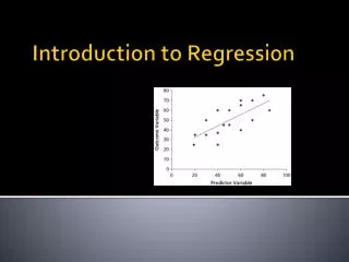
Regression • A statistical method used to examine the relationship between a variable of interest (dependent variable) and one or more explanatory variables (predictors) • Strength of the relationship • Direction of the relationship (positive, negative, zero) • Goodness of model fit • Allows you to calculate the amount by which your dependent variable changes when a predictor variable changes by one unit (holding all other predictors constant) • Often referred to as Ordinary Least Squares (OLS) regression • Regression with one predictor is called simple regression • Regression with two or more predictors is called multiple regression • Available in all statistical packages • Just like correlation, if an explanatory variable is a significant predictor of the dependent variable, it doesn’t imply that the explanatory variable is a cause of the dependent variable
Example • Assume we have data on median income and median house value in 381 Philadelphia census tracts (i.e., our unit of measurement is a tract) • Each of the 381 tracts has information on income (call it Y) and on house value (call it X). So, we can create a scatter-plot of Y against X. • Through this scatter plot, we can calculate the equation of the line that best fits the pattern (recall: Y=mx+b, where m is the slope and b is the y-intercept) • This is done by finding a line such that the sum of the squared (vertical) distances between the points and the line is minimized • Hence the term ordinary least squares • Now, we can examine the relationship between these two variables
We can easily extend this to cases with 2+ predictors • When we have n>1 predictors, rather than getting a line in 2 dimensions, we get a line in n+1dimensions (the ‘+1’ accounts for the dependent variable) • Each independent variable will have its own slope coefficient which will indicate the relationship of that particular predictor with the dependent variable, controlling for all other independent variables in the regression. • The equation of the best fit line becomes where • The coefficient βof each predictor may be interpreted as the amount by which the dependent variable changes as the independent variable increases by one unit (holding all other variables constant)
An Example with 2 Predictors: Income as a function of House Value and Crime
Some Basic Regression Diagnostics • The so-called p-value associated with the variable • For any statistical method, including regression, we are testing some hypothesis. In regression, we are testing the null hypothesis that the coefficient (i.e., slope) βis equal to zero (i.e., that the explanatory variable is not a significant predictor of the dependent variable). • Formally, the p-value is the probability of observing the value of β as extreme (i.e., as different from 0 as its estimated value is) when in reality it equals to zero (i.e., when the Null Hypothesis holds). If this probability is small enough (generally, p<0.05), we reject the null hypothesis of β=0 for an alternative hypothesis of β<>0. • Again, when the null hypothesis (of β=0) cannot be rejected, the dependent variable is not related to the independent variable. • The rejection of a null hypothesis (i.e., when p <0.05) indicates that the independent variable is a statistically significant predictor of the dependent variable • One p-value per independent variable
Some Basic Regression Diagnostics (Cont’d) • The sign of the coefficient of the independent variable (i.e., the slope of the regression line) • One coefficient per independent variable • Indicates whether the relationship between the dependent and independent variables is positive or negative • We should look at the sign when the coefficient is statistically significant (i.e., significantly different from zero)
Some Basic Regression Diagnostics (Cont’d) • R-squared (AKA Coefficient of Determination): the percent of variance in the dependent variable that is explained by the predictors • In the single predictor case, R-squared is simply the square of the correlation between the predictor and dependent variable • The more independent variables included, the higher the R-squared • Adjusted R-squared: percent of variance in the dependent variable explained, adjusted by the number of predictors • One R-squared for the regression model
Some (but not all) regression assumptions • The dependent variable should be normally distributed (i.e., the histogram of the variable should look like a bell curve) • Ideally, this will also be true of independent variables, but this is not essential. Independent variables can also be binary (i.e., have two values, such as 1 (yes) and 0 (no)) • The predictors should not be strongly correlated with each other (i.e., no multicollinearity) • Very importantly, the observations should be independent of each other. (The same holds for regression residuals). If this assumption is violated, our coefficient estimates could be wrong! • General rule of thumb: 10 observations per independent • variable
N=140 An Example of a Normal Distribution
Data Transformations • Sometimes, it is possible to transform a variable’s distribution by subjecting it to some simple algebraic operation. • The logarithmic transformation is the most widely used to achieve normality when the variable is positively skewed (as in the image on the left below) • Analysis is then performed on the transformed variable.
Additional Regression Methods • Logistic regression/Probit regression • When your dependent variable is binary (i.e., has two possible outcomes). • E.g., Employment Indicator (Are you employed? Yes/No) • Multinomial logistic regression • When your dependent variable is categorical and has more than two categories • E.g., Race: Black, Asian, White, Other • Ordinal logistic regression • When your dependent variable is ordinal and has more than two categories • E.g., Education: (1=Less than High School, 2=High School, 3=More than High School) • Poisson regression • When your dependent variable is a count • E.g., Number of traffic violations (0, 1, 2, 3, 4, 5, etc)
Spatial Autocorrelation • Recall: • There is spatial autocorrelation in a variable if observations that are closer to each other in space have related values (Tobler’s Law) • One of the regression assumptions is independence of observations. If this doesn’t hold, we obtain inaccurate estimates of the β coefficients, and the error term ε contains spatial dependencies (i.e., meaningful information), whereas we want the error to not be distinguishable from random noise.
Imagine a problem with a spatial component… This example is obviously a dramatization, but nonetheless, in many spatial problems points which are close together have similar values
But how do we know if spatial dependencies exist? • Moran’s I (1950) – a rather old and perhaps the most widely used method of testing for spatial autocorrelation, or spatial dependencies • We can determine a p-value for Moran’s I (i.e., an indicator of whether spatial autocorrelation is statistically significant). • For more on Moran’s I, see http://en.wikipedia.org/wiki/Moran%27s_I • Just as the non-spatial correlation coefficient, ranges from -1 to 1 • Can be calculated in ArcGIS • Other indices of spatial autocorrelation commonly used include: • Geary’s c (1954) • Getis and Ord’s G-statistic (1992) • For non-negative values only
So, when a problem has a spatial component, we should: • Run the non-spatial regression • Test the regression residuals for spatial autocorrelation, using Moran’s I or some other index • If no significant spatial autocorrelation exists, STOP. Otherwise, if the spatial dependencies are significant, use a special model which takes spatial dependencies into account.
Spatial Regression Models • A spatial lag (SL) model • Assumes that dependencies exist directly among the levels of the dependent variable • That is, the income at one location is affected by the income at the nearby locations • A “lag” term, which is a specification of income at nearby locations, is included in the regression, and its coefficient and p-value are interpreted as for the independent variables. • As in OLS regression, we can include independent variables in the model. • Whereas we will see spatial autocorrelation in OLS residuals, the SL model should account for spatial dependencies and the SL residuals would not be autocorrelated, • Hence the SL residuals should not be distinguishable from random noise (i.e., have no consistent patterns or dependencies in them)
OLS Residuals vs. SL Residuals Non-random patterns and clustering Random Noise
But how is spatial proximity defined? • For each point (or areal unit), we need to identify its spatial relationship with all the other points (or areal units). This can be done by looking at the (inverse of the) distance between each pair of points, or in a number of other ways: • A binary indicator stating whether two points (or census tract centroids) are within a certain distance of each other (1=yes, 0=no) • A binary indicator stating whether point A is one of the ___ (1, 5, 10, 15, etc) nearest neighbors of B (1=yes, 0=no) • For areal datasets, the proportion of the boundary that zone 1 shares with zone 2, or simply a binary indicator of whether zone 1 and 2 share a border (1=yes, 0=no) • Etc, etc, etc • When we have n observations, we form an n x n table (called a weight matrix or a link matrix) which summarizes all the pairwise spatial relationships in the dataset • These weight matrices are used in the estimation of spatial regression (and the calculation of Moran’s I). • Unless we have compelling reasons not to do so, it’s generally a good idea to see whether our results hold with different types of weight matrices
Assume we have a map with 10 Census tracts The hypothetical weight matrix below indicates whether any given Census tract shares a boundary with another tract. 1 means yes and 0 means no. For instance, tracts 3 and 6 do share a boundary, as indicated by the blue 1’s.
Now, we need a software package that can… • Run the good old OLS regression model • Create a weight matrix • Test for spatial autocorrelation in OLS residuals • Run a spatial lag model (or some other spatial model) Such packages do exist!
GeoDa • A software package developed by Luc Anselin • Can be downloaded free of charge (for members of educational and research institutions) at https://www.geoda.uiuc.edu/ • Has a user-friendly interface • Accepts ESRI shapefiles as inputs • Is able to perform a number of basic GIS operations in addition to running the sophisticated spatial statistics models
Other Spatial Regression Models • Spatial Error (can be implemented in GeoDa) • Geographically-Weighted Regression (can be run in ArcGIS 9.3) These methods also aim to account for spatial dependencies in the data
Some References: Spatial Regression • Bailey, T.C. and Gatrell, A.C. (1995). Interactive Spatial Data Analysis. Addison Wesley Longman, Harlow, Essex. • Cressie, N.A.C. (1993). Statistics for Spatial Data. (Revised Edition). Wiley, John & Sons, Inc. • LeSage, J. and Pace K.R. (2009). Introduction to Spatial Econometrics. CRC Press/Taylor & Francis Group.