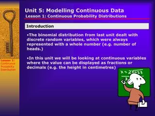
Unit 5: Modelling Continuous Data
Unit 5: Modelling Continuous Data. Lesson 1: Continuous Probability Distributions. Introduction. The binomial distribution from last unit dealt with discrete random variables, which were always represented with a whole number (e.g. number of heads.)

Unit 5: Modelling Continuous Data
E N D
Presentation Transcript
Unit 5: Modelling Continuous Data Lesson 1: Continuous Probability Distributions Introduction • The binomial distribution from last unit dealt with discrete random variables, which were always represented with a whole number (e.g. number of heads.) • In this unit we will be looking at continuous variables where the value can be displayed as fractions or decimals (e.g. the height in centimetres) Lesson 1: Continuous Probability Distribution
Unit 8: The Normal Distribution Lesson 1: Continuous Probability Distributions • Continuous Variables – • Normal Distribution • Assembly times for 36 tricycles • How can we make the histogram Continuous? • Discrete Variables – • Binomial Distribution • The number of head tossed when a coin is tossed 5 times Lesson 1: Continuous Probability Distribution
Unit 8: The Normal Distribution Lesson 1: Continuous Probability Distributions Continuous Probability Distributions • As stated above the variables that we will focus on are those of the continuous nature • Let us now examine a special case: • Investigate and Inquire • The table below gives the failure rates for a model of computer printer during its first four years of use. Lesson 1: Continuous Probability Distribution
Unit 8: The Normal Distribution Lesson 1: Continuous Probability Distributions • Construct a scatter plot of these data. Use the midpoint of each interval. Sketch a smooth curve that is good fit to the data • Why do you think printer failure rates would have this shape of distribution? • Calculate the mean and the standard deviation of the failure rates. How useful are these summary measures in this distribution? Lesson 1: Continuous Probability Distribution
Unit 8: The Normal Distribution Lesson 1: Continuous Probability Distributions • Calculating Standard Deviation and Mean: Lesson 1: Continuous Probability Distribution
Unit 8: The Normal Distribution Lesson 1: Continuous Probability Distributions The mean printer life is 24 months, with a standard deviation of 14.7 months. These summary measures are not very useful in describing the distribution, since so many data points lie far from the mean. How can this data be represented? Using a continuous curve of best fit. Lesson 1: Continuous Probability Distribution
Unit 8: The Normal Distribution Lesson 1: Continuous Probability Distributions Terminology of Continuous Distributions Positively Skewed – A distribution with no symmetry and is pulled to the right Lesson 1: Continuous Probability Distribution Negative Skewed – A distribution with no symmetry and is pulled to the left
Unit 8: The Normal Distribution Lesson 1: Continuous Probability Distributions Unimodal – The examples above are unimodal since they only contain one “hump”. This is similar to the mode of a set of discrete values. Bimodal - Contains two “humps”. For example the speed in the 100 m for Olympic athletes would have two “humps” since it would contain different times for males and females. Lesson 1: Continuous Probability Distribution
Unit 8: The Normal Distribution Lesson 1: Continuous Probability Distributions Example 1-Uniform Continuous Distributions • Suppose the commuting time form Georgetown to downtown Toronto varies uniformly from 30 to 55 minutes, depending on traffic and weather conditions. Construct a graph of this distribution and use the graph to find: • The probability that a trip takes 45 minutes or less. • The probability that a trip takes more than 48 minutes. Lesson 1: Continuous Probability Distribution • We know that every time from 30 to 55 min is equally likely to occur • The distribution would be a horizontal line since this is uniform • The area under the line must equal 1 since each time is equally likely to occur and the total probability is 1. • The probability of each event to occur can be found by its interval: This means that the likelihood that you would arrive in Toronto at any time from 30 – 55 minutes is 4%.
Prob. Density Prob. Density 0.04 0.04 45 55 55 30 30 Minutes Minutes Unit 8: The Normal Distribution Lesson 1: Continuous Probability Distributions The distribution graph is a uniform one Lesson 1: Continuous Probability Distribution a) The graph for less than 45 minutes would look like the yellow shade below: P(Time<45) = 0.04(45-30) =0.6 or 60%
Prob. Density 0.04 48 55 30 Minutes Unit 8: The Normal Distribution Lesson 1: Continuous Probability Distributions b) The graph for greater than 48 minutes would look like the yellow shade below: P(Time>48) = 0.04(55-48) =0.28 or 28% Lesson 1: Continuous Probability Distribution
Unit 8: The Normal Distribution Lesson 1: Continuous Probability Distributions Lesson 1: Continuous Probability Distribution