Download
1 / 50
530 likes | 1.11k Vues
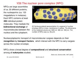
V26 The nuclear pore complex (NPC). NPCs are large assemblies of ca. 30 different proteins, the nucleoporins (ca. 120 megadaltons in metazoa). Each NPC contains at least 456 individual protein molecules. They mediate the

E N D
V26 The nuclear pore complex (NPC) NPCs are large assemblies of ca. 30 different proteins, the nucleoporins (ca. 120 megadaltons in metazoa). Each NPC contains at least 456 individual protein molecules. They mediate the bidirectional exchange of macromolecules between the nucleus and the cytoplasm. (E) Surfacerendered representation of a segment of nuclear envelope (NPCs in blue, membranes in yellow). The dimensions of the rendered volume are 1680 nm 984 nm 558 nm. The number of NPCs was ca. 45/m2. Nucleocytoplasmic transport of macromolecular cargoes depends on their recognition by transport factors, which interact with the NPC to carry cargoes across the nuclear envelope. NPCs show a broad degree of compositional and structural conservation among all eukaryotes studied. Beck et al. Science 306, 1387 (2004) Bioinformatics III
The nuclear pore complex Structure of the Dictyostelium NPC. (A). Cytoplasmic face of the NPC in stereo view. The cytoplasmic filaments are arranged around the central channel; they are kinked and point toward the CP/T. (B) Nuclear face of the NPC in stereo view. The distal ring of the basket is connected to the nuclear ring by the nuclear filaments. (C) Cutaway view of the NPC with the CP/T removed. Beck et al. Science 306, 1387 (2004) Bioinformatics III
Alber et al., Nature 450, 683 (2007) Bioinformatics III
Nuclear Pore Complex EM studies in several organisms have revealed that the general morphology of the NPC is conserved. These studies show the NPC to be a doughnut-shaped structure, consisting of 8 spokes arranged radially around a central channel that serves as the conduit for macromolecular transport. Each NPC spans the nuclear envelope through a pore formed by the fusion of the inner and outer nuclear envelope membranes. Numerous filamentous structures project from the NPC into the cytoplasm and nucleoplasm. Bioinformatics III
4-level hierarchical representation of the NPC In the NPC, we consider 30 protein types (nups) and their relative stoichiometries, leading to a total of 456 protein molecules. CryoEM shows the NPC as a ring with an eight-fold rotational axis perpendicular to the NE plane. This symmetry indicates that the NPC is composed of 8 identical building blocks, termed spokes. ImmunoEM experiments localized each nup to the nucleoplasmic, cytoplasmic, or both sides of the equatorial plane formally represent the NPC composition and protein stoichiometry with a 4-level hierarchy, consisting of - the whole NPC (assembly, A), - the half spoke (unit, U), - the nup (protein, P), - and bead (particle, B) levels. Each of the eight half-spoke units U at the cytosolic side is composed of 27 different types of nups, of which two are present in two copies each, totaling 29 protein instances. Similarly, each of the eight half-spoke units U at the nucleoplasmic side contains 28 protein instances of 25 different types. Bioinformatics III
Protein representation Every protein P is represented as a set of beads B, each with associated attributes (e.g., radius, mass). The number of beads and their attributes determine the resolution (granularity) of the protein representation. The most detailed data about the shape of most nups come from hydrodynamic experiments approximate the coarse shape and volume of each protein with a linear chain of equally-sized beads that best reproduce the observed sedimentation coefficients and are also consistent with our fold assignments. Protein conformations in the NPC may differ from their conformations in solution. Therefore each protein is represented as a flexible chain, to allow for maximally extended to maximally compact conformations (“Protein chain restraint”). The bead chain describes a protein at the highest resolution in our representation (the “root” representation κ = 1). Bioinformatics III
Bead representations Bioinformatics III
Protein representation As a convenient way of further representing their structure, each protein can be described by several additional representations κ that are derived from the “root” representation, but capture different aspects about the structural and biological properties of the protein. E.g. representation κ = 2 contains only beads corresponding to protein regions with defined native structures, representation κ = 3 represents the same regions with a single bead per protein. Here, we used up to 9 representations per protein that are used simultaneously. Each representation consists of a set of particles Bjκ and their attributes, such as the particle radii, partial protein mass, and the Cartesian coordinates. Except for the “root” representation (κ = 1), the attributes of a particle are fully or partly derived from particle attributes of another representation of the same protein. E.g. the Cartesian coordinates of all particles in representations κ from 2 to 9 are calculated from the particle coordinates in κ = 1, either by inheriting the coordinates from one of the particles in the root representation or by averaging the positions of some or all particles in the root representation. A configuration of the assembly is defined by the specific values of the particle attributes of all particles in B. Bioinformatics III
Overview of integrative structure determination Our approach to structure determination can be seen as an iterative series of 4 steps: - data generation by experiment, - translation of the data into spatial restraints, - calculation of an ensemble of structures by satisfaction of these restraints, and - an analysis of the ensemble to produce the final structure. The structure calculation part of this process is expressed as an optimization problem, a solution of which requires three main components: (1) a representation of the assembly in terms of its constituent parts; (2) a scoring function, consisting of individual spatial restraints that encode all the data; and (3) an optimization of the scoring function, which aims to yield structures that satisfy the restraints. Bioinformatics III
Analogy to NMR spectroscopy Formally, this approach is similar to the determination of protein structures by NMR spectroscopy, in which the folding of the polypeptide chain is determined by satisfying distance restraints between pairs of atoms. As with NMR spectroscopy, a structure is computationally determined from experimental data. Here, atoms are replaced by proteins, and their positions and relative proximities are restrained on the basis of data from a variety of proteomics and other experiments, including affinity purification, ultracentrifugation, electron microscopy and immuno-electron microscopy (immuno-EM). Bioinformatics III
Data generation: NPC component list To determine any structure, we must first define its parts. NPC is assembled from some 30 nucleoporins. Although the exact composition is still uncertain because some proteins interact relatively transiently with the NPC, potential omission of a small fraction of such transient components is unlikely to interfere with structure determination. Figure 2 Structural representation of the NPC. a, Hierarchical representation of the NPC that facilitates the expression of the experimental data in terms of spatial restraints. Formally, we define the whole NPC assembly A as a set of symmetry units U of two different types with 8 instances each, referred to as half-spokes. Half-spokes of the first type (green) reside at the cytoplasmic side and half-spokes of the second type (red) reside at the nucleoplasmic side of the nuclear envelope. Two adjacent half-spokes, one of each type, form a spoke. Each of the 16 NPC half-spokes consists of a set of proteins P that are described by their type and index. Each protein is represented by a flexible string of beads B in the root representation = 1. Additional representations > 1 can be derived from the root representation (for example, by omitting some beads as in = 2 or by combining beads as in = 3). For the NPC, each protein is described with up to 9 different representations. Bioinformatics III
Dimensions and symmetry b, Top panel: the dimensions of the nuclear envelope, as taken from cryo-EM images. Bottom-left panel: the coordinate system we use has the origin at the centre of the nuclear envelope pore. The nuclear envelope is indicated in grey. Bottom-right panel: the eight-fold (C-8) and two-fold (C-2) symmetry axes of the NPC, as revealed primarily by cryo-EM. We apply the two-fold symmetry only to proteins that appear with identical stoichiometry in both the nucleoplasmic and cytoplasmic half-spokes. Bioinformatics III
Stochiometry of each component in the NPC Identification of Nup82 copy number. Aliquots of NE preparations from PrA tagged strains equivalent to 3.6, 6, 10 and 15 μg were processed for immunoblot analysis. The strains with known copy number – Nup42, Nup1 (1 copy per spoke), Nup57, Nup84, Nup85 (2 copies per spoke) and Nsp1 (4 copies per spoke) were used as a control. Themembranes were probed first with MAb118C3 to detect Pom152 (the internal standard) and then with HRP conjugated IgG to detect both MAb118C3 and the PrA tag. Shown here are the slope values for each Nup, with value for Nup82 falling into the same range as the values of the 2 copy per spoke Nups. Bioinformatics III
Shape and size of each component Because atomic structures have not yet been solved for most nucleoporins, we estimated their shapes based primarily on their sedimentation coefficients determined by ultracentrifugation of the purified proteins. The sedimentation behaviour of most FG nucleoporins agrees with their predicted filamentous, native disordered structure. Pom152, an integral membrane component, appeared to be a highly elongated structure, consistent with its multiple domains modelled as b-cadherin-like folds. Most of the other nucleoporins appear to have a relatively compact tertiary structure that is again in agreement with their predicted fold assignments. The seven-protein Nup84 complex13 could be separated into two smaller complexes on sedimentation: an elongated tetramer (composite 30) and an elongated hexamer (composite 45), consistent with their elongated appearance when visualized by EM. Bioinformatics III
Protein shape from hydrodynamic experiments Purified native PrA-tagged nucleoporins were sedimented on sucrose gradients, together with a set of biotin-labelled marker proteins. Fractions were collected and analysed by immunoblotting of the biotin and PrA tags. An immunoblot of fractions from a typical sedimentation analysis is shown, indicating the position of the tagged protein (Nup159–PrA) together with the markers ovalbumin (3.6 S), bovine serum albumin (4.3 S), alcohol dehydrogenase (ADH, 7.4 S) and b-amylase (8.9 S). Bioinformatics III
Protein shape from hydrodynamic experiments Peak positions for the sedimenting proteins were determined and linear regression was used to calibrate the sedimentation coefficients of the PrA-tagged nucleoporin. Bioinformatics III
Protein shape from hydrodynamic experiments Bead representations = 1 of the NPC proteins and their stoichiometries per half-spoke. The stoichiometry of a protein in the cytoplasmic (cyt.) and nucleoplasmic (nucl.) half-spoke, as measured by quantitative immunoblotting, is shown. Smax values were calculated based on the molecular mass (kDa) of each protein; Smax/Sobs < 1.4 indicates a globular protein; 1.6–1.9, moderately elongated; > 2, highly elongated. asterisk: C-terminal fragments were measured. Also shown is a visualization of the protein as a flexible bead chain (shown here in its most extended configuration), which is based on sedimentation analysis, identification of domains by sequence comparison and secondary structure prediction. Bioinformatics III
Size, shape and symmetry of the NPC It is also helpful to have some information on the overall shape and symmetry of the NPC. The position of the nuclear envelope membrane relative to the NPC and the NPC’s symmetry are based on EM and cryo-EM data. These revealed an 8-fold rotational symmetry of the yeast NPC and an roughly 2-fold rotational symmetry between the nucleoplasmic and cytosolic halves of the NPC, defining the ‘half-spoke’ as a 16-fold pseudo-symmetry unit of the NPC. We have also previously shown that heparin treatment of isolated NPCs produced a ring-like substructure (‘Pom rings’), which is associated with the pore membrane and perinuclear space in the intact NPC. We isolated and examined these rings, and found that they had a maximum diameter of ca. 106 nm, consistent with the measured maximum NPC diameter of ca. 97nm. Bioinformatics III
Localization of each component in the NPC The coarse localization of most nucleoporins within the NPC was obtained by immuno-EM, relying on a gold-labelled antibody that specifically interacted with the localized protein through its carboxy-terminal PrA tag. Figure 4 | Localization of proteins by immuno-EM. a) Immuno-EM montages for Pom152–PrA nuclei and Ndc1–PrA nuclear envelopes. Scale bars are graduated in 10-nm intervals using the coordinate system defined in Fig. 2b. The major features in each montage are shown schematically at the right, showing how the position of every gold particle in each montage was measured from both the central Z-axis of the NPC (R) and from the equatorial plane of the nuclear envelope (Z). Bioinformatics III
Localization of each component in the NPC More accurate and complete immunolocalization map of the NPC Estimated position of the C terminus of each protein in the NPC relative to the central Z-axis of the NPC (R) and the equatorial plane (Z) superimposed on the protein density map of a cross-section of the yeast NPC obtained by cryo-EM. The average allowed ranges along the R and Z coordinates (68nm and 64.5 nm, respectively) are indicated by the brown bars in the bottom right corner. Bioinformatics III
Localization of each component in the NPC Inherent limitations in the immuno-EM method allow it to provide only a broad range of allowed axial and radial values for each nucleoporin. Nevertheless, these ranges are smaller than the dimensions of the half-spoke and so are still informative. Notably, most nucleoporins are found on both the nuclear and cytoplasmic sides of the NPC and are tightly packed within a region adjacent to the nuclear membrane. Most of the FG nucleoporins are found on both sides of the NPC, with a small number found exclusively on the cytoplasmic or nuclear side; for simplicity, we consider Nup116 and Nup100 to be cytoplasmically disposed and Nup145N to be nucleoplasmically disposed, although ca. 20% of the signal of each is found on the opposite side. Most of the non-FG nucleoporins are also found on both sides. The membrane proteins are found close to the nuclear envelope membrane, and Pom152–PrA is localized to the lumen of the nuclear envelope. Bioinformatics III
How do the NPC components fit together? The coarse shape, approximat position and stoichiometry of each nucleoporin are not enough to build an accurate picture of the NPC: rather like the pieces in a jigsaw puzzle, we also need information on the interactions between nucleoporins. We obtained this information from a large number of overlay assays and affinity purification experiments, as well as from the composition of the Pom rings (consisting of Pom34 and Pom152). An overlay assay identifies a pair of proteins that interact with each other, whereas an affinity purification identifies one or more proteins that interact directly or indirectly with the bait protein. An affinity purification produces a distinctive set of co-isolating proteins, which we term a composite. A composite may represent a single complex of physically interacting proteins or a mixture of such complexes overlapping at least at the tagged protein. Bioinformatics III
Protein interactions of the Nup84 complex Bioinformatics III
Protein interactions of the Nup84 complex Figure 5. a, A sample of affinity purifications containing Nup84 complex proteins. Affinity-purified PrA-tagged proteins and interacting proteins were resolved by SDS–PAGE and visualized with Coomassie blue. The name of the PrA-tagged protein together with a corresponding identification number for the composite is indicated above each lane. Molecular mass standards (kDa) are indicated to the left of the panel. The bands marked by filled circles at the left of the gel lanes were identified by mass spectrometry. The identity of the co-purifying proteins is indicated in order below each lane; PrA-tagged proteins are indicated in blue, co-purifying nucleoporins in black, NPC-associated proteins in grey, and other proteins (including contaminants) in red. b, The mutual arrangement of the Nup84-complex-associated proteins as visualized by their localization volumes. The localization volumes, obtained from the final NPC structure (Fig. 9), allow a visual interpretation of the relative proximities of the proteins. Bioinformatics III
Localization of each component in the NPC A good example of the compositional overlap is the Nup84 complex (Fig. 5a, b). The smallest building blocks of this complex are heterodimers (Fig. 5, composites 7, 14, 15). Under different isolation conditions, these dimers can be purified with an increasing number of additional proteins, such as trimers (25, 20), a tetramer (33), a pentamer (39), hexamers (44, 45, 51), and the full septameric Nup84 complex (53, 54, 57). This full complex interacts with Nup157 (63, 66) and Nup145N (60). Finally, the entire Nup84 complex coprecipitates together with the Nup170 complex and an Nsp1-containing complex (79). Bioinformatics III
Figure 6 | Protein proximity by affinity purification. a, Composites determined by affinity purification. The affinity-purified nucleoporin–PrA is indicated on the vertical axis, and the corresponding nucleoporins in each composite are shown on the horizontal axis. Composite identifiers are indicated to the right. Presence of a nucleoporin in a composite is indicated by a black box, and the tagged nucleoporin is indicated by a light grey box. In composite 64 (Pom152) and in composites 31 and 61 (Nup82), a second untagged copy of a corresponding protein is present, indicated by a black box. Dark grey box: a direct interaction determined by overlay assay. The asterisk for Nup84 indicates that the data were obtained with GFP-tagged Nup84. Bioinformatics III
b, Distributions of composite size (left) and composite similarity (right). The similarity between two composites is defined by 2a / (2a + b + c), where a is the number of proteins that occur in both composites, b is the number of proteins present only in the first composite, and c is the number of proteins present only in the second composite. Bioinformatics III
Restraints and the scoring function Structure determination is enabled by expressing information as a scoring function, the global optimum of which corresponds to the structure of the native assembly. One such function is a joint probability density function (PDF) of protein positions, given the available information I about the system, p(C/I), where C = (c1 ,c2,…,cn ) is the list of the cartesian coordinates (ci) of the n component proteins in the assembly (that is, the configuration of the proteins). This joint PDF gives the probability density that a component i of the native configuration is positioned very close to ci, given the information I we wish to consider in the calculation. In general, I may include any structural information from experiments, physical theories, or statistical preferences. Bioinformatics III
Restraints and the scoring function The complete joint PDF is generally unknown, but can be approximated as a product of PDFs pf that describe individual assembly features (for example, distances or relative orientations of proteins): The scoring function F(C) is then defined as the logarithm of the joint For convenience, we refer to the logarithm of a feature PDF as a restraint rf and the scoring function is therefore the sum of the individual restraints. Bioinformatics III
Ambiguity in data interpretation Figure 7 | Ambiguity in data interpretation and conditional restraints. a, The ambiguity for a protein interaction between proteins of green and yellow types is illustrated. The ambiguity results from the presence of multiple copies of the same protein in the same or neighbouring symmetry unit. In our NPC calculations, both neighbouring half-spokes on the cytoplasmic and nucleoplasmic sides are considered, for a total of four neighbouring half-spokes (not shown). Bioinformatics III
b, The conditional restraint is illustrated by an example of a composite of four protein types (yellow, blue, red, green), derived from an assembly containing a single copy of the yellow, blue, and red protein and two copies of the green protein; proteins are represented by a single bead (blue protein), a pair of beads (green and red proteins), and a string of three beads (yellow protein) (right panel). This composite implies that at least 3 of the following 6 possible types of interaction must occur: blue–red, blue–yellow, blue–green, red–green, red–yellow and yellow–green. In addition, (1) the 3 selected interactions must form a ‘spanning tree’ of the ‘composite graph’; (2) each type of interaction can involve either copy of the green protein; and (3) each protein can interact through any of its beads. These considerations can be encoded through a tree-like evaluation of the conditional restraint. At the top level, all optional bead–bead interactions between all protein copies are clustered by protein types. Each alternative bead interaction is restrained by a harmonic upper bound on the distance between the beads; these are ‘optional restraints’, because only a subset is selected for contribution to the final value of the conditional restraint. Next, a ‘rank-and-select’ operator (ORS) selects only the least violated optional restraint from each interaction type, resulting in six restraints (thick red line) at the middle level of the tree. Finally, the minimal spanning tree operator (OMST) finds the combination of 3 restraints that are most consistent with the composite data (thick red line); here the edge weights in the minimal spanning tree correspond to the restraint values given the current assembly structure. The column on the right shows a structural interpretation of the composite with proteins represented by their coloured beads and alternative interactions indicated by edges between them. The composite graph (left) is a fully connected graph that consists of nodes for all identified protein types and edges for all pairwise interactions between protein types; in the context of the conditional restraint, the edge weights correspond to the restraint values. 5 of the 16 possible spanning trees are also shown. This restraint evaluation process is executed at each optimization step based on the current configuration, thus resulting in possibly different subsets of selected optional restraints at each step. Bioinformatics III
Calculation of the NPC bead structure by satisfaction of spatial restraints a, Representation of the optimization process as it progresses from an initial random configuration to an optimal structure. The graph shows the relationship between the score (a measure of the consistency between the configuration and the input data) and the average contact similarity. The contact similarity quantifies how similar 2 configurations are in terms of the number and types of their protein contacts; a contact between two proteins occurs if the distance between their closest beads is less than 1.4 times the sum of the bead radii. Representative configurations at various stages of the optimization process from left (very large scores) to right (with a score of 0) are shown above the graph; a score of 0 indicates that all input restraints have been satisfied. As the score approaches zero, the contact similarity increases, showing that there is only a single cluster of closely related configurations that satisfy the input data. Bioinformatics III
Definition of potential protein interactions Supplementary Figure 13: Definition of potential protein interactions. The list of all alternative interactions (thick lines) between protein instances of type = α and β defined for proteins in half-spokes Us=1θ=1 (dark unit, upper row) and Us=1θ =2 (dark unit, lower row). Left column: All pairwise combinations of proteins of type α in Usθ (red circles) with all potential interaction partners of type β in half-spokes Us′θ′ with (θ′,s′) ∈N(θ,s) (below). Middle column: all combinations of proteins of type β in Usθ (red circles) with all potential interaction partners of type α in half-spokes Us′θ′ , where (θ′, s′) ∈N(θ,s). Right column: all possible interactions Iαβ (θ,s) between proteins of type α and β for half-spoke Usθ defined as the union of both groups Bioinformatics III
Conditional protein interactions Bioinformatics III
Simulation protocol Bioinformatics III
Optimization in two stages First, a coarse sampling protocol (left column) generates 200,000 coarse configurations, starting each time from a different random configuration. This protocol relies on a variable target function method that consists of gradually increasing the number of restraints that are included in the scoring function, finally culminating in the full scoring function F. At each stage of the variable target function method, a combination of the conjugate gradient (CG) minimization and a molecular dynamics (MD) simulation with simulated annealing is applied. In total, a single optimization of an initial random configuration consists of an iteration of approximately 10.000 small shifts of protein particles (guided by either CG or MD). Second, a refinement protocol (right column) further refines the best 10% configurations from the sampling stage. Bioinformatics III
Bead model, ensemble, localization probability Bioinformatics III
Bead model, ensemble, localization probability a, Top: 2 representative bead models of the NPC (excluding the FG-repeat regions) from the ensemble of 1,000 superposed structures satisfying all restraints. The 8 positions of 3 sample proteins (Nup192, Nup57 and Nup85) on the cytoplasmic side are shown, with a detailed view of the bead representation of 1 copy of Nup85 at the bottom. Bioinformatics III
Bead model, ensemble, localization probability b, The localization probability for each protein type is obtained by converting the ensemble into the probability of any volume element being occupied by the protein. Shown are contourmaps of the cross-sections in the plane parallel to the equatorial plane that contains the maximum value of the protein localization probability. Bioinformatics III
Bead model, ensemble, localization probability c, The localization volume of the sample proteins, derived from the localization probability. The volume elements are first sorted by their localization probability values. The localization volume then corresponds to the top-ranked elements, the volume of which sums to the protein volume, estimated from its molecular mass. The localization volume of a protein reveals its most probable localization. Because of the limited precision of the information used here, the localization volume of a protein should not be mistaken for its density map, such as that derived by cryo-EM. Bioinformatics III
Bead model, ensemble, localization probability Figure 10 | Ensemble interpretation in terms of protein positions, contacts and configuration. a, Localization volumes of all 456 proteins in the NPC (excluding the FG-repeat regions) in 4 different views. The diameter of the transport channel and the NPC are also indicated. The proteins are colour-coded according to their assignment to the 6 NPC modules. Bioinformatics III
Bead model, ensemble, localization probability b, Contact frequencies for all pairs of proteins. The contact frequency of a pair of protein types is the fraction of structures in the ensemble that contains at least one protein contact between any protein instances of the two types. Bioinformatics III
Bead model, ensemble, localization probability c, Contact frequencies between proteins in composite 40. Proteins are nodes connected by edges with the observed contact frequency as the edge weight (indicated by its thickness). Edges that are part of the maximal spanning tree are shown by thick blue lines; the maximal spanning tree is the spanning tree that maximizes the sum of the edge weights. All edges with a statistically significant reduction in contact frequency from their initial values implied by the composite data alone (P-value <10-3) are indicated by dotted lines with contact frequencies shown in red. Bioinformatics III
Bead model, ensemble, localization probability d, Protein adjacencies for the whole NPC, with proteins as nodes and edges connecting proteins that are determined to be adjacent to each other. The edge weight is the observed contact frequency. Bioinformatics III
Bead model, ensemble, localization probability e, Configuration of the proteins in composite 40. The location of a protein corresponds to the average position of the beads representing non-FG repeats of the protein. f, Configuration of Nic96 and the NPC scaffold proteins. g, Localization volume of Nic96 and the NPC scaffold proteins. Bioinformatics III
Bead model, ensemble, localization probability Figure 11 | The structure is increasingly specified by the addition of different types of synergistic experimental information. a, Protein positions. As an example, each panel illustrates the localization of 16 copies of Nup192 in the ensemble of NPC structures, generated using the data sets indicated below. The localization probability is contoured at 65% of its maximal value (red). The smaller the volume, the better localized are the proteins. The NPC structure is therefore essentially moulded into shape by the large amount of diverse experimental data. Bioinformatics III
Protein contacts Contact frequencies reflect the likelihood that a protein interaction is formed given the data considered and are calculated from the ensemble of optimized structures. Prediction of protein interactions from contact frequencies improves as more data are used. This figure shows as an example the contact frequencies between proteins found in composite 34. Contact frequencies are shown as edge weights and indicated by the thickness of the lines connecting the proteins. Left: when only a single composite is used (together with stoichiometry and symmetry information), all interactions are equally likely. Middle: when the highest likelihood of interaction between a particular protein pair from all composites is used, the uncertainty about the interactions is reduced. Right: when all data are used, the contact frequencies are either very high (>0.65) or very low (<0.25), thus allowing a strong prediction of protein interactions. Numbers in red indicate final contact frequencies that significantly decreased (at a P-value <10-3) from their initial values. Bioinformatics III
Evaluation by experimental data not used sofar Finally, our structure can be tested by comparing it to experimental data that were not included in the structure calculation. 1 omission of a randomly chosen subset of 10% of the protein interaction data still results in structures with contact frequencies essentially identical to those derived from the complete data set the structure is robust. 2 the shape of our NPC structure strongly resembles the published EM maps of the NPC, even though these data were not used here. 3 the diameter of the transport channel in our structure is ca. 38nm (excluding the FG-repeat regions), in good agreement with the experimentally reported maximal diameter of transported particles. 4 Nup133, which has been experimentally shown to interact with highly curved membranes via its ALPS-like motif, is adjacent to the nuclear envelope in our structure. 5 perhaps the best example is that of the Nup84 complex. Our configuration for this complex is completely consistent with previous results. Together these assessments indicate that our data are sufficient to determine the configuration of the proteins comprising the NPC. Indeed, it is hard to conceive of any combination of errors that could have biased our structure towards a single solution that resembles known NPC features in so many ways. Bioinformatics III
Conclusions We have devised an integrative approach to solve the structure of the NPC using diverse biophysical and proteomic data. This approach has several advantages: 1 it benefits from the synergy among the input data. Data integration is in fact necessary for structure determination, because none of the individual data sets contains sufficient spatial information on its own. 2 the integrative approach can potentially survey all the structures that are consistent with the data. Alternatively, if no structure is consistent with the data, then some experiments or their interpretations are incorrect. 3 this approach can make the process of structure determination more efficient, by indicating which measurements would be most informative. 4 the approach can, in principle, incorporate essentially any structural information about a given assembly. Thus, it is straightforward to adapt it for calculating higher resolution structures by including additional spatial restraints from higher resolution data sets, such as atomic structures of proteins, chemical crosslinking, footprinting, small angle X-ray scattering (SAXS) and cryo-EM. These additional data sets might allow us to determine pseudo-atomic structures of assemblies as complex as the NPC. The molecular architecture of many macromolecular complexes could, in principle, be resolved using a similar integrative approach. Bioinformatics III