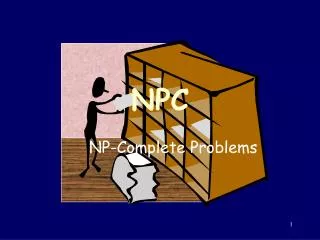
NPC

1. NPC NP-Complete Problems

2. We can solve any problem(!)(?) • …but perhaps not with a computer! • Some problems are not computable: • The Halting Problem: Write a function boolean halts(Program p, Input i); which returns true if p halts on input i, and false if it doesn’t. • A bonus homework exercise?

3. If we could write the halts function, then we could also write: boolean loopIfHalts(Program p, Input i) { if (halts(p,i)) while (true) ; else return true; } boolean testSelf(Program p) { return loopIfHalts(p,p); } • What is testSelf(testSelf)?

4. boolean halts(Program p,Input i); which returns true if p halts on input i, and false if it doesn’t. boolean loopIfHalts(Program p, Input i) { if (halts(p,i)) while (true) ; else return true; } boolean tS(Program p) {return loopIfHalts(p,p); } Assume: tS(tS) halts and returns true. loopIfHalts(tS,tS) = true halts(tS,tS) = false tS(tS) doesn't halt which is a contradiction Assume: tS(tS) does not halt halts(tS,tS) = true contradiction Proof by contradiction:

5. We can solve any computable problem! • …but perhaps not with an “efficient” algorithm. • Of course we could solve any problem by: • Enumerating all possible solutions; • Testing each one to see if it is a solution. • That may take a long time … • … but sometimes it seems that’s the best we can do!

6. x1 x2 x3 Circuit Satisfiability: • Find an assignment of truth values to the inputs of a logic circuit, that results in an output of 1.

7. Hamiltonian Cycles: • Given a graph G, find a simple cycle that contains each vertex in G.

8. Subset Sum: • Given a finite set of natural numbers S and a target natural number t, find a subset S’ of S whose sum is t. • For example, find: S’{1,3,6,34,93,243,654,1040,1436,1879} with sum S’ = 2361.

9. What is a problem? • Abstractly, a problem is a set of pairs (I,S), where I is an instance of the problem and S is a solution. • A decision problem is a problem in which the solutions are either yes or no. (i.e., 0 or 1) • An optimization problem O is a subset of a problem P in which, if (I,S)O and (I,S’)P, then SS’, with respect to some ordering . (I.e. the solution S is better than S')

10. Decision Problems: • To solve a decision problem on a computer: • Provide the computer with an instance; • Wait for a yes/no answer. • In most cases, we will need to encode the instance in a form that the computer can manipulate. • We will assume that instances are coded as strings of bits: i.e., by elements of {0,1}*

11. General picture: Encodings, e Abstract Problems Concrete Problems For example: Does e(G) represent a connected graph? Is G a connected graph?

12. Problem Solving: • An algorithm solves a problem in time O(T(n)) if, for any instance I, the algorithm can produce a solution S in time O(T(|I|)). • A problem is polynomial-time solvable if there is an algorithm to solve it in time O(nk), for some constant k.

13. Polynomial time = Tractable? • The computable polynomial-time algorithms that we encounter in practice usually have relatively low values of k. • The set of polynomial-time problems is the same in many reasonable models of computation. • The set of polynomial-time algorithms has nice closure properties.

14. P The set of concrete decision problems that are solvable in polynomial time.

15. Encodings, e Abstract Problems Concrete Problems Polynomial Time Solvability for Abstract Algorithms: • We would like to extend these ideas to abstract algorithms: • An abstract decision problem Q is solvable in polynomial time if the encoding e(Q) is in P. • This depends on the encoding used!

16. Not all encodings are equal! • Suppose we have A(k) = (k) • for example: A(k) = 1+2+3+ ... +k • If we code the integer k in binary notation, then we require n = log k bits of input. • If we code an integer k in unary notation, then we require n = k+1 bits of input. • Then algorithm A will have: • Exponential complexity, (2n), if we use the binary representation; • Linear complexity, (n), if we use the unary representation.

17. This seems counter intuitive: • The "better" the encoding the worse the complexity! • In reality the same work is happening in both cases, we just inflated the size of the input (in the unary encoding) so the complexity appears better. • Moral of the Story: If comparing two Abstract decision problems be sure the two encodings you are using are comparable!

18. {0,1}* e1 Instances e2 {0,1}* Relating Encodings: • A function f : {0,1}*{0,1}* is polynomial-time computable if there is an algorithm that, given any input x, produces f(x) as output in polynomial time. • Encodings e1 and e2 are polynomially related if there are polynomial-time computable functions f and g mapping between them. g f

19. If e1 and e2 are polynomially related encodings on the instances of an abstract decision problem Q, then: e1(Q)P  e2(Q)P • So, as long as we stick to reasonable, concise encodings, the exact encoding doesn’t alter our ability to solve a problem in polynomial time.

20. Accepting and Deciding: • Given a string x{0,1}*, an algorithm A: • accepts x, if it outputs 1 given input x. • rejects x, if it outputs 0 given input x. • decides x, if it either accepts or rejects x. • is there another choice? • A language is a set of strings x{0,1}*. • The set of strings x{0,1}* for which an algorithm A outputs 1 is called the language accepted by A. • Similar definitions for the languages rejected or decided by an algorithm …

21. Languages correspond to concrete decision problems: • The language for a problem Q is just the set of strings that have solution 1. • In this setting, P is the set of all problems that can be decided in polynomial time.

22. This is the same as the set of languages that can be accepted in polynomial-time! • Suppose L can be accepted in polynomial time by an algorithm A. Then A will accept L after at most cnk steps for some constants c, k. • To decide L in polynomial time, simulate cnk steps in the execution of A. (A polynomial time overhead.) If it hasn’t terminated with an answer after that many steps, then it won’t ever be accepted, and so we can return 0.

23. Write down 5 problems that are in P: • How many decision problems can you think of that are not in P?

24. Verifying Solutions: • It is often much easier to verify that a given value is a solution of a problem, than it is to calculate a solution directly. • A verification algorithm takes two inputs: • A string x, representing a problem instance; • A string y, called a certificate. • Algorithm A verifies a language L if L is precisely the set of strings xL for which there exists a certificate y such that A(x,y) returns 1.

25. NP stands for non-deterministic polynomial NP The set of concrete decision problems that are verifiable in polynomial time.

26. “Nondeterministic Polynomial”: • If a decision problem is in NP, then we can calculate solutions for an instance x by: • Enumerating all possible answers y; • Verifying each one using A(x,y) until we find a solution. • If there are N possible solutions, this will take O(Nnk) time. But often N is O(cn), and so the overall time is O(cn) too (since cn grows much faster than nk as n goes to infinity). • The best case time is O(nk) --- if the first answer we try is a solution.

27. P NP: • If L is in P, then we can construct a polynomial-time verification algorithm A(x,y) that simply ignores the certificate y, and accepts precisely those strings that it determines to be in L. • Is P=NP? After more than three decades, this is still an open question … but many researchers believe that they are not equal.

28. Reductions

29. Motivation • Reductions are our main tool for comparison between problems.

30. Introduction • Objectives: • To formalize the notion of “reductions”. • Overview: • Karp reductions • HAMPATH p HAMCYCLE • Closeness under reductions • Cook reductions • Completeness

31. Reductions – Concept IF we can translate problem A to problem B… A B p THENB is at least as hard as A.

32. SIP 250 I.e – there exists a polynomial time TM which halts with f(w) on its tape when given input w. Reductions – Formal Definition Definition: Language A is polynomial time reducible to language B if… a polynomial time computable function f:** exists, Denote: A p B where for every w, wA  f(w)B f is called the polynomial time reduction of A to B.

33. B f * - B * Reductions and Algorithms A * - A *

34. Reductions and Algorithms polynomial time algorithm for A f polynomial time algorithm for B f(w)B? f(w) wA? w

35. How to Reduce? • Construct f. • Show f is polynomial time computable. • Prove f is a reduction, i.e show: • If wA thenf(w)B • If f(w)B thenwA

36. Terminology • The type of reductions we’ve just described is also called: • Polynomial-time mapping reduction • Polynomial-time many-one reduction • Polynomial-time Karp reduction • We’ll always refer to such reductions unless otherwise specified.

37. Example • To demonstrate a reduction, we’ll revisit the example we gave in the introduction. • We’ll rephrase and formalize the seating and tour problems • And demonstrate a slightly different reduction between them.

38. Hamiltonian Path Instance: a directed graph G=(V,E) and two vertices stV. Problem: To decide if there exists a path from s to t, which goes through each node once. In the version presented in the introduction we asked for some path, without specifying the start and end vertices.

39. Hamiltonian Cycle Instance: a directed graph G=(V,E). Problem: To decide if there exists a simple cycle in the graph which goes through each node exactly once.

40. n s s t t HAMPATH pHAMCYCLE f( <G=(V,E),s,t> ) = <G’=(V{u},E{(u,s),(t,u)})> f( <G=(V,E),s,t> ) = <G’=(V{u},E{(u,s),(t,u)})> f( <G=(V,E),s,t> ) = <G’=(V{u},E{(u,s),(t,u)})> f( <G=(V,E),s,t> ) = <G’=(V{u},E{(u,s),(t,u)})> p

41. Correctness • (Completeness) If there exists a Hamiltonian path (v0=s,v1,…,vn=t) in the original graph, then (u,v0=s,v1,…,vn=t,u) is a Hamiltonian cycle in the new graph.

42. Correctness • (Soundness)(u,s) and (t,u) must be in any Hamiltonian cycle in the constructed graph, thus removing u yields a Hamiltonian path from s to t.

43. How to Reduce?  • Construct f. • Show f is polynomial time computable. • Prove f is a reduction, i.e show: • If wHAMPATH thenf(w)HAMCYCLE • If f(w)HAMCYCLE thenwHAMPATH  easy to verify   

44. Closeness Under Reductions Definition: A complexity class C is closed under reductions if, whenever L is reducible to L’ and L’C, then L is also in C. C L’  L

45. Observation Theorem:P, NP, PSPACE and EXPTIME are closed under polynomial-time Karp reductions. Proof: Filling in the exact details is left to the reader. (See sketch)

46. Other Types of Reductions • Cook Reduction: Use an efficient “black box” (procedure) that decides B, to construct a polynomial-time machine which decides A. polynomial time algorithm for B polynomial time algorithm for A

47. Cook reduction of HAMCYCLE to HAMPATH. • For each edge (u,v)E, • if there’s a Hamiltonian path from v to u in the graph where (u,v) is removed, output ‘YES’, exit • Output ‘NO’ Make sure it’s efficient! HAMPATH oracle

48. Reducibility: • Problem Q can be reduced to problem Q’ if every instance of Q can be rephrased as an instance of Q’. • A language L1 is polynomial-time reducible to a language L2, written L1P L2, if there is a polynomial-time computable function f such that: x  L1 f(x)  L2 • f is a reduction function; an algorithm that computes f is a reduction algorithm.

49. x F f(x) A2 f(x)L2 xL1 Reduction algorithm Algorithm for deciding L2 Algorithm for deciding L1 • If L1P L2 and L2 is in P, then so is L1.

50. NP-completeness: • A language L is NP-complete if: • L is in NP; and • L’P L for every L’ in NP. A language that satisfies just this property is said to be NP-hard.